Computing Isogenies between Montgomery Curves Using the
Action of (0
,
0)
Joost Renes?
Digital Security Group, Radboud University, Nijmegen, The Netherlands
Abstract. A recent paper by Costello and Hisil at Asiacrypt’17 presents efficient formulas for computing isogenies with odd-degree cyclic kernels on Montgomery curves. We provide a con-structive proof of a generalization of this theorem which shows the connection between the shape of the isogeny and the simple action of the point (0,0). This generalization removes the restric-tion of a cyclic kernel and allows for any separable isogeny whose kernel does not contain (0,0). As a particular case, we provide efficient formulas for 2-isogenies between Montgomery curves and show that these formulas can be used in isogeny-based cryptosystems without expensive square root computations and without knowledge of a special point of order 8. We also consider elliptic curves in triangular form containing an explicit point of order 3.
Keywords: V´elu’s formulas, Montgomery form, 2-isogenies, SIDH, Post-quantum cryptogra-phy.
1 Introduction
Ever since their introduction to public-key cryptography by Miller [Mil86] and Koblitz [Kob87], elliptic curves have been of interest to the cryptographic community. By using the group of points on an appropriately chosen elliptic curve where the discrete logarithm problem is as-sumed to be hard, many standard protocols can be instantiated. Notably, the Diffie–Hellman key exchange [DH76] and the Schnorr signature scheme [Sch89] and its variants [Acc99,
BDL+12] allow for efficient implementations with high security and small keys. The efficiency of these curve-based algorithms is largely determined by the scalar multiplication routine, and as a result a lot of research has gone into optimizing this operation.
However, the threat of large-scale quantum computers has initiated the search for al-ternative algorithms that also resist quantum adversaries (which the classical curve-based systems do not [Sho94]). Building on the work of Couveignes [Cou06] and Rostovsev and Stolbunov [RS06], in 2011 Jao and De Feo [JF11] proposed supersingular isogeny Diffie– Hellman (SIDH) as a key exchange protocol offering post-quantum security. Being based on the theory of elliptic curves, SIDH inherits several operations from traditional curve-based cryptography. As such, it has immediately benefited from decades of prior research into op-timizing their operations. In particular, the Montgomery form of an elliptic curve has re-sulted in great performance. Initially proposed by Montgomery to speed up factoring using ECM [Mon87, Len87] and having been used for very efficient Diffie–Hellman key exchange (eg. Bernstein’s Curve25519 [Ber06]), the current fastest instantiations of SIDH also employ Montgomery curves [CLN16b,KAK16]. But, although the optimizations for scalar multiplica-tion immediately carry over, the work on computing explicit isogenies on Montgomery curves is more limited.
?This work has been supported by the Technology Foundation STW (project 13499 – TYPHOON &
For isogeny computations one commonly uses V´elu’s formulas [V´el71]. However, if the elliptic curve has a form which is less general than (or different from) Weierstrass form, the formulas from V´elu are not guaranteed to preserve this. As isogenies are only well-defined up to isomorphism, one can post-compose with an appropriate isomorphism to return to the required form, but it may not be obvious with which isomorphism, or the isomorphism may be expensive to compute. A more elegant approach is to observe some extra structure on the curve model and require the isogenies to preserve this. For example, Moody and Shumow [MS16] apply this idea to Edwards and Huff curves by fixing certain points. Moreover, since the isogeny is invariant under addition by kernel points, there is a close connection between the isogeny and the action (by translation) of some chosen point. We make this more explicit in Theorem1for curves in Weierstrass form.
So far the approaches for obtaining formulas for isogenies on Montgomery curves have been rather ad hoc. In [FJP14], De Feo, Jao and Plˆut apply V´elu’s formulas and compose with the appropriate isomorphisms to return to Montgomery form. As noted in [FJP14, §4.3.2], this approach fails to produce efficient results for 2-isogenies. That is, either one has to compute expensive square roots in a finite field (see eg. [CJL+17, §3.1]), or one relies on having an appropriate point of order 8. However, this point of order 8 is not readily available for the final two 2-isogenies. As one suggested workaround in [FJP14] they derive formulas for 4-isogenies between two curves in Montgomery form and propose to compute 2e-isogenies as a chain of 4-isogenies. As a result, optimized SIDH implementations [CLN16a, KAK16] have employed curves whereeis even so that 2e-isogenies can be comprised entirely of 4-isogenies. In [CH17], Costello and Hisil present elegant formulas for isogenies between Montgomery curves, but their theorem covers only the case of odd cyclic kernels and subsequently also does not address the case of 2-isogenies. Moreover, there is no justification for the derivation of these isogenies (except for showing that they work).
We bridge this gap by providing a more thorough analysis on isogenies between Mont-gomery curves. We show that the isogenies arising in [CH17] are exactly those fixing (0,0). Since we enforce the isogeny to fix (0,0), this point cannot be in the kernel. We show in Propo-sition 1 that this is the only restriction, and as a result present a generalization of [CH17, Theorem 1]. As a special case, we obtain formulas for 2-isogenies for 2-torsion points other than (0,0). We then show that this point can be naturally avoided in well-designed isogeny-based cryptosystems (see §4.3), and discuss the application of the 2-isogeny formulas to isogeny-based cryptosystems.
Finally, although currently it does not give rise to faster isogeny formulas, we consider it worthwhile to point out that the same techniques immediately apply to other models. In particular, models derived from the Tate Normal Form[Hus04,§4.4], where one could expect to get simple`-isogenies for`≥3. We work out the case`= 3, also known as thetriangular form [BCKL15], and derive isogenies by again fixing the action of the special point (0,0).
2 Preliminaries
An elliptic curveE defined over a field K is by definition [Gal12,Sil09] the curve
E/K :Y2Z+a1XY Z+a3Y Z2=X3+a2X2Z+a4XZ2+a6Z3 , (1)
wherea1, a2, a3, a4, a6 ∈K such thatE is non-singular. It is embedded intoP2 with a single
point OE = (0 : 1 : 0) on the line Z = 0. This form is commonly referred to as Weierstrass form and the specified base point (implicitly) isOE. On the open patch defined by Z 6= 0 we can setx=X/Z andy=Y /Z and work on the corresponding affine curve insideA2 given by
E/K :y2+a1xy+a3y =x3+a2x2+a4x+a6 .
We can move back to the projective curve by mapping (x, y)7→(x:y : 1). Therefore, although many equations are given in affine coordinates, they can easily be transformed into projective ones. For any extensionL/K, the set ofL-rational points E(L) forms a group with identity
OE [Sil09, Prop. 2.2(f)]. A subgroupG⊂E( ¯K) is said to be defined overK ifσ(P)∈Gfor allσ in the Galois group Gal( ¯K/K).
Isogenies. LetE andEebe elliptic curves. An isogenyφfromEtoEeis a surjective morphism such that φ(OE) = OEe [Sil09, §III.4]. The (finite) degree d of an isogeny is its degree as a
morphism, and we say an isogeny is separable if # ker(φ) = d. In this paper every isogeny that appears is assumed to be separable. Given a finite subgroup G ⊂ E( ¯K) defined over K, there exists a curve Ee and an isogeny φ : E → Ee such that ker(φ) = G [Gal12, Theo-rem 9.6.19]. The curve Ee is unique up to isomorphism (over ¯K) and the isogenyφ is unique up to post-composition with an isomorphism. The isogeny φ can be made explicit by using V´elu’s formulas [V´el71] (for some fixed choice for the isogeny).
Montgomery Form. Setting a1 = a3 = a6 = 0 and a4 = 1 gives a curve in the form
E:y2=x3+ax2+x. We also consider curves in the formby2 =x3+ax2+x, better known
as Montgomery form. Over ¯K these two curve forms are isomorphic via (x, y) 7→ (x, y√b), but this isomorphism is only defined overK if√b∈K. In particular, if K=Fq and
√
b /∈K then we call this curve a (non-trivial) quadratic twist. An easy check shows thatQ= (0,0) is a K-rational point of order 2, while for anyQ4 ∈E( ¯K) we have that [2]Q4 =Qif and only if
Q4∈ {(1,±
p
(a+ 2)/b),(−1,±p(a−2)/b)}
IfP is any point of order 2 other thanQ, thenx2P +axP + 1 = 0.
Tate Normal Form. Suppose we are given a curveE/K containing a pointP of prime order `≥3. We can move P to (0,0) and its tangent line to the line y= 0. This transformation is completelyK-rational and puts the curve inTate Normal Form [Hus04,§4.4]
y2+axy+by=x3+cx2, a, b, c∈K .
In§5 we focus on the case where`= 3, in which case c = 0 and b6= 0. Moreover, ifb=β3, then the transformation (x, y) 7→ (x/β2, y/β3) lets us assume that b= 1 and thus gives the form
Note thatβis not necessarily defined overK. However, Proposition4shows that once we start on such a curve, the 3-isogenies will preserve this form. It has discriminant∆(E) =a3−27 and has a subgroup {OE,(0,0),(0,−1)} of order 3. The point (0,0) acts on points outside this subgroup by
(x, y) + (0,0) = −
y x2,
−y x3
.
This curve is known as atriangular curve [BCKL15] and is isomorphic to the twisted Hessian curve [BCKL15, Theorem 5.3]
(a3−27)x3+y3+ 1 = 3axy .
SIDH. Let eA, eB, f ∈ Z≥0 such that p = `eAA` eB
B f −1 is prime. For K = Fp2 we can then find a supersingular curveE overK [Br¨o09] such that
#E(K) = (p+ 1)2 , E(K)[`eA
A ] =Z/` eA
A Z×Z/` eA AZ , E(K)[`eB
B ] =Z/` eB
B Z×Z/` eB B Z . By having the two parties compute isogenies of degree`eA
A resp. ` eB
B and composing we can define a key exchange algorithm [FJP14,§3.2] similar to Diffie–Hellman. Since these degrees are exponentially large, they cannot be computed directly by polynomial evaluation. Instead, we decompose an`eA
A -isogeny as a sequence ofeA isogenies of degree`A, which are efficiently computable for small`A [FJP14,§4] (typically`A∈ {2,3}). Focusing on one of the sides, the secret key is a tuple (γ, δ) ∈ Z/`eA
A Z×Z/` eA
A Z where not both γ and δ are divisible by `A. Fixing a basisE(K)[`eA
A ] =hP, Qi, this corresponds to an isogeny with kernelh[γ]P + [δ]Qi. As the kernel is determined by its generator up to some invertible scalar multiple, and since at least one of the two scalars must be invertible, all keys can either be put in the form (1, δ) or (γ,1).
3 Isogenies on Weierstrass Curves
We begin by stating a straightforward, but rather useful theorem. By assuming to have knowledge on the action of an isogeny on a single point Q, we can translate this point by elements of the kernel to obtain a simple description of the isogeny. Many curve models have a natural choice for this point (eg.Q= (0,0) in Montgomery form, see §4).
Theorem 1. Let K be a field andE/K an elliptic curve in Weierstrass form. LetG⊂E( ¯K) be a finite subgroup defined over K and
φ: (x, y)7→(f(x), c0yf0(x) +g(x)), c0 ∈K¯∗ , (2)
a separable isogeny such thatker(φ) =G. Let Q∈E( ¯K) such that Q /∈G. Then
f(x) =c1(x−xQ)
Y
T∈G\{OE}
(x−xQ+T)
Proof. First note that the existence ofφfollows from V´elu’s formulas [V´el71], while a standard result [Gal12, Theorem 9.7.5] shows that it can be written in the form of (2) (where f0(x) is the formal derivative df /dx of f(x)). More explicitly, following the notation of [Gal12, Theorem 25.1.6], there exist functionsu, t:G\ {OE} →K¯ such that
f(x) =x+ X T∈G1∪G2
t(T) x−xT
+ u(T) (x−xT)2
,
whereG2⊂Gis the set of points of order 2 and G1⊂E( ¯K) is such that
G={OE} ∪G2∪G1∪ {−T :T ∈G1} .
Moreover,u(T) = 0 if and only ifT has order 2. Collecting denominators, it is then immediate that there exists a functionw∈K[x] such that deg(w) =¯ |G|and
f(x) = w(x)
v(x) , wherev(x) = Y
T∈G\{OE}
(x−xT) .
Now define
h(x) =w(x)v(xQ)−w(xQ)v(x) .
Note that clearlyh(xQ) = 0. Since the value off is invariant under the action of points inG, we in fact have that h(xQ+T) = 0 for allT ∈G. Therefore it follows that (x−xQ+T) |h(x) for all T ∈ G. If for all T1, T2 ∈ G such that T1 =6 T2 we have that xQ+T1 6=xQ+T2, then it immediately follows that
Y
T∈G
(x−xQ+T)|h(x) .
Otherwise1, assume we have T1, T2 ∈ G such that T1 =6 T2 and xQ+T1 = xQ+T2. Since any x-coordinate corresponds to at most 2 points on E, it follows that Q+T2 = ±(Q+T1).
However,Q+T2 =Q+T1 implies thatT1=T2, which contradicts our assumption. Therefore
Q+T2 =−(Q+T1) and
[2]φ(Q+T1) =φ(Q+T1) +φ(Q+T1)
=φ(Q+T1) +φ(Q+T2)
=φ(Q+T1)−φ(Q+T1)
=O
e
E . Moreover,
[2](Q+T1) =OE ⇐⇒ Q+T1+Q+T1 =OE
⇐⇒ Q+T1−(Q+T2) =OE
⇐⇒ T1=T2 ,
which contradicts the assumption that T1 6= T2. Thus ψ2(Q+T1) 6= 0 and by Lemma 1 we
can conclude thatf0(xQ+T1) = 0. Since away from the zeros of v we have h(x) = f(x)−f(xQ)
v(x)v(xQ) , 1
it follows from the fact thatf0(xQ+T1) =f(xQ+T1)−f(xQ) = 0 thath0(xQ+T1) = 0. That is, hhas (at least) a double root at xQ+T1. In other words,
(x−xQ+T1)(x−xQ+T2)|h(x) .
It is then clear that indeed
Y
T∈G
(x−xQ+T)|h(x) .
As deg(h)≤max(deg(w),deg(v)) =|G|, there exists a constant c∈K∗ such that
h(x) =c Y T∈G
(x−xQ+T) .
Thus,
f(x) = w(x) v(x) =
h(x)
v(x)v(xQ) +f(xQ) .
The result follows by settingc1 =c/v(xQ). ut
Lemma 1. Let the setup be as in Theorem 1 and let R∈E( ¯K)\G. Then
[2]φ(R) =O
e
E ⇐⇒ ψ2(R)f
0(x
R) = 0 , where ψ2 is the 2-division polynomial.
Proof. Firstly note thatR /∈Gand thusφ(R)6=O
e
E. Therefore, by definition of the 2-division polynomial onEe=E/Git follows that
[2]φ(R) =O
e
E ⇐⇒ 2yφ(R)+ea1xφ(R)+ea3 = 0 ,
whereea1 andea3 are Weierstrass constants of Ee conform (1). Using the definition ofφand by recalling that (see eg. [Gal12, Theorem 9.7.5])
2g(xR) =c0(a1xR+a3)f0(xR)−ea1f(xR)−ea3 ,
a straightforward computation shows that
2yφ(R)+ea1xφ(R)+ea3= 0 ⇐⇒ c0(2yR+a1xR+a3)f
0(x
R) = 0 .
Finally observe thatψ2(R) = 2yR+a1xR+a3 and c0 6= 0. ut
Remark 1. Theorem 1 shows the connection between φ and the action of the point Q on abscissas of kernel elements, asφ is given by a product of functions
x−xQ+T x−xT .
Remark 2. By relying on Theorem1 we simplify the proof compared to earlier works [CH17,
MS16]. Whereas those works present rational maps and prove them to be isogenies, we turn this argument around. We use the existence of the isogeny (by V´elu’s formulas) and apply appropriate isomorphisms to enforce some structure to be maintained (eg. (0,0)7→ (0,0) in Montgomery form). We can then apply Theorem1to get formulas for the isogeny up to some constants. Finally we also use the formal group law. However, as opposed to proving that the rational functions defining the isogeny satisfy the curve relation of the co-domain curve, we can assume them to vanish and therefore extract the constants and the coefficients of the co-domain curve. This significantly simplifies the proof compared to earlier works (eg. [MS16, Theorem 2] and [CH17, Theorem 1]).
4 Montgomery Form and 2-isogenies
In [CH17, Theorem 1] Costello and Hisil present rational maps which they prove to be isogenies between Montgomery curves. These isogenies are not unique, and are for example different from the formulas directly derived using V´elu’s formulas. It is immediate that the isogenies in [CH17] have the property of fixing (0,0). In§4.1we show that this fact, together with the co-domain curve being in Montgomery form, characterizes their formulas (up to some sign choices). This generalizes the theorem by Costello and Hisil, by removing the restriction of kernels being cyclic and having odd order. In particular, in§4.2 we present formulas for 2-isogenies determined by points of order 2 other than (0,0). Until now these had not appeared, and were considered to require the computation of a square root. In §4.3 we show how one could apply these formulas in an implementation. Although it requires only a modest change to the parameters, this does require care and can simplify the implementation. Finally in§4.4
we comment on a comparison to the state-of-the-art.
4.1 The General Formula
We begin by stating Proposition 1, which is the analogue of [CH17, Theorem 1].
Proposition 1. Let K be a field with char(K)6= 2. Let a∈K such that a2 6= 4 and E/K :
y2 = x3 +ax2 +x is a Montgomery curve. Let G ⊂ E( ¯K) be a finite subgroup such that (0,0) ∈/ G and let φ be a separable isogeny such that ker(φ) = G. Then there exists a curve
e
E/K :y2 =x3+Ax2+x such that, up to post-composition by an isomorphism,
φ:E →Ee
(x, y)7→(f(x), c0yf0(x))
where
f(x) =x Y T∈G\{OE}
xxT −1 x−xT
.
Moreover, writing
π= Y T∈G\{OE}
xT , σ= X T∈G\{OE}
xT − 1
xT
,
Proof. Over ¯K we can always move E/G to Montgomery form. Let P ∈ E( ¯K) such that xP = 1. Then [2]P = (0,0), hence [2]φ(P) = φ([2]P) 6= OE/G while [4]φ(P) = [2] (0,0) =
OE/G. Thusφ(P) is a point of exact order 4, and we apply an isomorphism such thatxφ(P)=
(−1)|G|−1 (see eg. [FJP14,§4.3.2]). In particular this assures thatφ: (0,0)7→(0,0). We then twist they-coordinate via another isomorphism to set the coefficient ofy2 to 1 and have
e
E=E/G:y2=x3+Ax2+x .
Now apply Theorem 1 withQ= (0,0). We obtain that
f(x) =c1(x−x(0,0))
Y
T∈G\{OE}
(x−x(0,0)+T) (x−xT)
+f(x(0,0))
=c1x
Y
T∈G\{OE}
x− 1
xT
(x−xT) .
As we set up Ee such that f(1) = (−1)|G|−1, we find that
c1 =
Y
T∈G\{OE} xT .
Feedingc1 back into the equation forf puts it in the right form. At this point it only remains
to findA and c0 (observe that g= 0 in Montgomery form [Gal12, Theorem 9.7.5]). To this
end we utilize the formal group law, similar to [CH17,MS16].
Lett=x/ybe a uniformizer atOE and writes= 1/y. By observing thats=t3+at2s+ts2 we can recursively substitutesinto itself to get an expressions(t)∈Z[a]JtKas a power series
2
s(t) =t3+at5+ (a2+ 1)t7+O(t9)
This is well-defined, see for example [Sil09,§IV.1]. As a result we can write
1/s(t) =y(t) =t−3−at−1+O(t) , ty(t) =x(t) =t−2−a+O(t2) .
LetX(t) =f(x(t)). Then
X(t) =πt−2+π(σ−a) +O(t2) , dX/dt=−2πt−3+O(t) ,
dx/dt=−2t−3+O(t) , (dx/dt)−1=−t3/2 +O(t7) .
Now define
Y(t) =c0y(t)·(df /dx)
=c0y(t)·(dX/dt)·(dx/dt)−1 ,
2
so that
Y(t) =c0πt−3−c0aπt−1+O(t) .
Writing
F(t) =Y(t)2− X(t)3+AX(t)2+X(t) it follows that
F(t) =F−6·t−6+F−4·t−4+O(t−2) ,
with
F−6=π2(c20−π), F−4 =π2 3π(a−σ)−2ac20−A
.
Now since by assumption φ is an isogeny with co-domain curve E, and sincee F is precisely the equation definingE, we must havee F = 0. Solving F−6 = 0 andF−4 = 0 simultaneously
leads to the desired equations for c20 and A. Note that this way we have only defined c0 up
to sign. However, the sign choice merely induces a composition with [−1] and therefore does
not affectφup to isomorphism. ut
Remark 3. It is perhaps not immediately obvious that Proposition1is a generalization of the result by Costello and Hisil [CH17, Theorem 1]. Our result assumes the domain curve E to be of the form y2 = x3 +ax2+x, while their theorem also accounts for curves E0 :by2 =
x3+ax2+x. Moreover, the map itself looks slightly different. However, it is straightforward to check that if one pre-composes with the isomorphism
ψ0:E0 →E
(x, y)7→(x, y√b) and post-composes with the isomorphism
ψ1 :Ee→E1:By2+x3+Ax2+x ,
(x, y)7→
x,√y
πb
then one recovers the theorem from Costello and Hisil in the case of odd-degree cyclic kernels. Ignoring these twists in Proposition1simplifies the proof. For example, see Proposition2. Remark 4. IfK=Fq is a (large-characteristic) finite field, then possiblyπ is a non-square in
Fq. As a result φis not defined over Fq. However, in that case the map
(x, y)7→(f(x), yf0(x))
is defined overFq with co-domain curveEe(t):πy2=x3+Ax2+x. This is the quadratic twist of E. Sincee Eeand its twist have the same Kummer line, we eliminate this issue by projecting toP1 (ie. by using x-only arithmetic).
Remark 5. If we set up an SIDH instance with `A = 2 and eA ≥ 2 then the x-coordinates of points of order 2 are in fact squares. This follows from [Hus04, Ch. 1, Thm 4.1] com-bined with the doubling formulas for Montgomery curves, as noted in [CJL+17, §3.2]. Since
4.2 2-isogenies
As an immediate consequence of Proposition1we obtain formulas for 2-isogenies for 2-torsion points other than (0,0).
Proposition 2. Let K be a field withchar(K)6= 2. Let a, b∈K such that b6= 0 anda2 6= 4, and E/K :by2 =x3+ax2+x is a Montgomery curve. Let P ∈ E( ¯K) such that P 6= (0,0) and [2]P =OE. Then
φ:E→E/Ke :By2 =x3+Ax2+x (x, y)7→(f(x), yf0(x)) ,
with B =xPb and A= 2(1−2x2P) is a 2-isogeny withker(φ) =hPi, where
f(x) =x·xxP −1
x−xP .
Proof. This is exactly the statement in Proposition 1 composed with the isomorphisms ψ0
and ψ1 from Remark 3. The result follows by using the identity axP =−(x2P + 1) to derive
A. ut
We also compute the kernel of the dual of φ, which will be helpful in §4.3 for larger degree isogenies.
Corollary 1. Let the setup be as in Proposition 2. Thenker(φ) =b h(0,0)i.
Proof. Letψbe a separable isogeny with domainEeand kernelh(0,0)i. Then certainlyE[2]⊂ ker(ψ◦φ), and since deg(ψ◦φ) = 4 we in fact have E[2] = ker(ψ◦φ). Thus ψ = φb up to isomorphism by uniqueness of the dual isogeny, and hence ker(φ) = ker(ψ).b ut The statement and proof of Proposition 2 does not explain why we are able to compute 2-isogenies without explicit square roots, while earlier works [CH17, FJP14] could not. We provide a more direct computation in Remark 6 to show why this is the case.
Remark 6. In [FJP14,§4.3.2] the authors describe a 2-isogeny with kernel (0,0) as ϕ:E →F :by2=x3+ (a+ 6)x2+ 4(2 +a)x
(x, y)7→
(x−1)2 x , y
1− 1
x2
.
The coefficient ofx can be removed by computing 2√a+ 2 and composing with the isomor-phism
(x, y)7→
x 2√a+ 2,
y 2√a+ 2
,
puttingF in the desired form. This requires computing a square root, which could be avoided by having knowledge of a pointP8 = 2
√
a+ 2,—
of order 8 above (0,0). Instead, we observe that we can compose with the isomorphism
ψ:F →G: √ b
a2−4y
2 =x3−√ 2a
a2−4·x 2+x
(x, y)7→
x+a+ 2
√
a2−4 ,
y
√
a2−4
which moves the kernel of ϕe to (0,0). This requires computing √a2−4 and therefore also
relies on a square root. However, ifP2= (x2,0) is a point of order 2 onE withx26= 0, then
x22+ax2+ 1 = 0. Therefore it is immediate that
p
a2−4 = 2x 2+a ,
allowing us to compute the isomorphism efficiently. We have such a point by assumption in Proposition 2. We can now compute φ asψ◦ϕ◦χ, where χ is an isomorphism mappingP2
to (0,0) (eg. [FJP14, Equation (15)]).
To provide explicit operation counts3 we move to projective space and project to P1. Let
P = (XP : 0 :ZP) be a point of order 2 onE:bY2Z=X3+aX2Z+XZ2 such thatXP 6= 0. Then by Proposition2
φ:E→Ee:BY2Z =X3+AX2Z+XZ2
(X: — :Z)7→(X(XXP −ZZP) : — :Z(XZP −ZXP))
is a 2-isogeny with kernelhPi. We have
A= 2 (ZP2 −2XP2)/ZP2 ,
and to avoid inversions we represent it projectively as
(A: 1) = (2 (ZP2 −2XP2) :ZP2) .
However, the doubling formulas on Montgomery curves use (A+ 2)/4 instead of A, and we see that
(A+ 2 : 4) = (ZP2 −XP2 :ZP2) . This can be computed in 2S+ 1a. Moreover, we observe that
X(XXP −ZZP) =X h
(X−Z)(XP +ZP)−(X+Z)(ZP −XP) i
,
Z(XZP −ZXP) =Z h
(X−Z)(XP +ZP) + (X+Z)(ZP −XP) i
.
This can be computed in 4M+ 6a via the sequence of operations
T0 =XP +ZP, T1 =XP −ZP, T2 =X+Z , T3 =X−Z , T4=T3·T0,
T5 =T2·T1, T6 =T4−T5, T7 =T4+T5, T8 =X·T6, T9 =Z·T7 .
If we assume XP +ZP and ZP−XP to be pre-computed, the cost reduces to 4M+ 4a. This would for example apply if we require multiple evaluations of the isogeny (eg. in SIDH). Also note that ZP2 −XP2 = (XP +ZP)(ZP −XP) which allows us to compute the curve coefficient in M+S. This may or may not be worth it, depending on the underlying architecture.
3 We denote byM,Sresp.athe cost of a field multiplication, squaring resp. addition or subtraction (which
4.3 Application to Isogeny-based Cryptography
In the general setting it is not true that the kernels appearing in the computations cannot con-tain the point (0,0), so it is not clear that the 2-isogenies can immediately be used. In a similar fashion, it is not true in general that kernels of 4-isogenies cannot contain (1,±p
(a+ 2)/b) or (−1,±p
(a−2)/b). In [CLN16a, §3] and [CH17] this assumption is used without justifi-cation (implicitly by replacing ψ4 with ψb4). This is dealt with by using a separate function
first 4 isog for the first 4-isogeny, which is the only kernel that can contain such a point (a proof of which does not appear). However, Lemma 2 and Corollary 2 show that we can avoid these points with only a minor restriction on the keyspace. Applying this restriction to [CLN16a] makes the functionfirst 4 isog redundant, simplifying the implementation.
Lemma 2. Let e, f ∈ Z≥0 and let p = 2e3f −1 be prime. Let E/Fp2 be a supersingular elliptic curve in Montgomery form such that #E(Fp2) = (p+ 1)2. Let P, Q ∈ E(Fp2) such that E[2e] =hP, Qi and [2e−1]Q= (0,0). Let α∈Z2e. Then (0,0)∈ h/ P + [α]Qi.
Proof. It is clear thathP+ [α]Qican only contain a single point of order 2, namely [2e−1](P+ [α]Q). But by assumption on Q we know that [2e−1](P + [α]Q) 6= (0,0), hence the result follows.
By Lemma 2 we know that we can compute the 2e-isogenies as defined in Proposition 1. However, as the degrees grow this will quickly be impractical. Instead, we do the computations as a sequence of 2-isogenies (ie. as in Proposition 2) [FJP14, §4]. Therefore we must show that none of these intermediate isogenies has a kernel generated by (0,0).
Corollary 2. Let the setup be as in Lemma 2 and writeR=P+ [α]Q. Let φ be an isogeny such thatker(φ) =hRi and suppose that we compute
φ=φe−1◦ · · · ◦φ0 ,
ker(φ0) =h[2e−1]Ri ,
ker(φi) =h
2e−i−1
φi−1· · ·φ0(R)i, (for 1≤i≤e−1)
as a sequence of2-isogenies, each one computed as in Proposition2. Then (0,0)∈/ ker(φi) for all0≤i≤e−1.
Proof. We apply induction on i. The statement for i= 0 follows from Lemma 2. Let i >0. Then ker(bφi−1) =h(0,0)i by the inductive hypothesis and by Corollary1. But since the walk
determined byφ is non-backtracking, it follows that ker(φi)6=h(0,0)i. As # ker(φi) = 2, we conclude that (0,0)∈/ ker(φi).
The keyspace is determined by tuples (γ, δ) which define kernels of the formh[γ]P + [δ]Qi, where not simultaneously γ ≡ 0 mod 2 and δ ≡ 0 mod 2. We can divide the space into the three disjoint sets (of equal size)
K(i,j)={(γ, δ) :γ≡imod 2, δ≡jmod 2} ,
Remark 7. The initial proposal to use curves in Montgomery form [CLN16a, §4] suggested taking P as an Fp-rational point on the curve E0/Fp :y2 =x3+x with j(E0) = 1728 and
Q as the image of P under the distortion map (x, y) 7→ (−x, iy). This allows a compressed representation of {P, Q}. Although this does not work for the basis as chosen in Lemma 2, it only results in a small increase in the size of public parameters (which never need to be transferred).
4.4 Relating 2-isogenies and 4-isogenies
It is easy to see that the 4-isogenies from [CH17, Appendix A], which are currently the fastest formulas, can be derived by applying the 2-isogenies from§4.2twice. That is, since they have equal kernel they are equal up to composition with an isomorphism. Both isogenies have a Montgomery curve as co-domain, of which there are at most six per isomorphism class (by looking at the formula for thej-invariant). Also, in both cases the dual is generated by a point P ∈ {(1,±p
(a+ 2)/b),(−1,±p
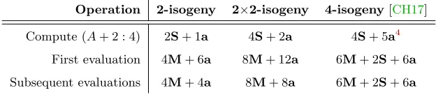
(a−2)/b)}. Therefore we can transform one into the other by possibly composing with the simple isomorphisms (x, y)7→(x,−y) and (x, y)7→(−x, iy), wherei∈K¯ such thati2 =−1. As a result, applying the 2-isogenies twice will not have more efficient formulas than the 4-isogenies. Indeed, if this were the case we could use the above transformation to obtain equally fast 4-isogenies. We summarize the costs in Table1.
Table 1.Comparison of the costs of evaluating 2-isogenies and 4-isogenies.
Operation 2-isogeny 2×2-isogeny 4-isogeny[CH17]
Compute (A+ 2 : 4) 2S+ 1a 4S+ 2a 4S+ 5a4
First evaluation 4M+ 6a 8M+ 12a 6M+ 2S+ 6a
Subsequent evaluations 4M+ 4a 8M+ 8a 6M+ 2S+ 6a
Besides their theoretic value, there are some small upsides to using 2-isogenies in an imple-mentation. Firstly, the computation leaks only a single bit as opposed to two [FJP14,§4.3.2]. Instead of leaking the dual of the final 4-isogeny, it would only leak the dual of the last 2-isogeny. Also, in some cases one may be able to select smaller parameters for a certain given security level. Primes of the form 2e3f −1 where e≈log2(3f) are somewhat sparse, and de-pending on one’s requirements restrictingeto be even could result in a (much) larger prime than hoped for. Alternatively, one could of course achieve this by doing a single 2-isogeny fol-lowed by a chain of 4-isogenies. However, this does come at the cost of having to implement more algorithms, increasing the size and complexity of an (already complex) implementa-tion. Finally, having worked out formulas for isogenies of even degree and by showing how to avoid (0,0), we are able to straightforwardly write down formulas for 2e-isogenies with e≥3. It remains to be seen if these can be made more efficient than repeated applications of 4-isogenies.
4
5 Triangular Form and 3-isogenies
Given the generality of Theorem 1, an obvious question is whether there are other classes of curves which could possibly give rise to simple formulas for isogenies. In this section we analyze curves in triangular formE/K:y2+axy+y=x3 containing a point (0,0) of order 3. Most of the ideas from earlier sections apply and in particular we get analogous statements for computing 3-isogenies (see§5.2). Although these allow to compute the co-domain curve very efficiently, the evaluation of the isogeny is not as efficient as its Montgomery counterpart. Moreover, since tripling formulas are currently slower, at this point Montgomery form still performs better with respect to 3-isogenies.
5.1 The General Formula
We start by presenting formulas for triangular curves that work for any separable isogeny whose kernel is an odd order subgroup. It is possible to include groups of even order, but this creates a case distinction which makes the proof more tedious. Since having (enough) rational points of even order would enable us to go to Montgomery form and reduce to§4, we discard that case here.
There are a couple of (minor) complications compared to the proof of Proposition 1. Firstly, we cannot assume that g= 0. If we work on P1 this will not affect the efficiency, but
we will have to take it into account in the proof. Secondly, the action of (0,0) does not involve only x-coordinates. To eliminate they-coordinates that arise, we group the kernel points into sets{T,−T} (similar to [CH17, Theorem 1]).
Proposition 3. Let K be a field with char(K) 6= 2. Let a ∈ K such that a3 6= 27 and E/K:y2+axy+y=x3 in triangular form. Let G⊂E( ¯K) be a finite subgroup of odd order
such that(0,0)∈/ Gand let φ be a separable isogeny such that ker(φ) =G. Let
X=
xP
P ∈G\ {OE}
.
Then there exists a curveE/Ke :y2+Axy+y=x3 such that, up to post-composition by an isomorphism,
φ:E→Ee
(x, y)7→(f(x), c0yf0(x) +g(x))
where
f(x) =xY z∈X
x2z2−x(az+ 1)−z (x−z)2 .
Moreover, writing
π= Y z∈X
z , σ =X z∈X
1 z2 +
a z −2z
,
Proof. Let P = (0,0). As φ(P) 6= OE/G, while [3]φ(P) = φ([3]P) = OE/G, it follows that φ(P) must have exact order 3 on E/G. Therefore by moving φ(P) to the origin we can put E/Gin triangular form and therefore assume that
e
E =E/G:y2+Axy+y=x3 .
Now apply Theorem 1 withQ=P. We find that
f(x) =c1(x−x(0,0))
Y
T∈G\{OE}
(x−x(0,0)+T) (x−xT)
+f(x(0,0))
=c1
Y
T∈G\{OE}
x+ yT x2 T
(x−xT)
=c1
Y
xT∈X
x+ yT x2 T
x+ y−T x2
T
(x−xT)2
=c1
Y
xT∈X
x2−x(axT+1) x2
T
−x1
T (x−xT)2
.
Observe that we use the fact that there are no points of order 2, and that
yTy−T =−x3T , and yT +y−T =−axT −1 .
By [Gal12, Theorem 9.7.5] we can write
g(x) = 1
2 −Af(x)−1 +c0axf
0(x) +c
0f0(x)
,
so thatg(0) = (−1 +c0f0(0))/2. Now we use the fact thatφ([2]P) = [2]φ(P), ie.φ: (0,−1)7→
(0,−1). Therefore
−1 =−c0f0(0) +g(0)
⇐⇒ −1 = −1−c0f0(0)
/2
⇐⇒c0= 1/f0(0)
⇐⇒c0= (−1)|X|π3/c1 . (3)
It remains to findA and c1 and for this we use the same strategy as earlier. Let t=x/y be
the uniformizer atOE and writes= 1/y. Then as a power series
s(t) =t3−at4+a2t5+O(t6) .
Asy= 1/s andx=ty we find that
LettingX(t) =f(x(t)) we get
X(t) =c1t−2+ac1t−1−c1σ+O(t) ,
dX/dt=−2c1t−3−ac1t−2+O(1) ,
dx/dt=−2t−3−at−2+O(t) ,
(dx/dt)−1 =−t3/2 +at4/4−a2t5/8 +O(t6) . It follows that
g(x(t)) = 1 2
−AX(t)−1 +c0·(dX/dt)·(dx/dt)−1·(ax(t) + 1)
= 1
2(ac0c1−Ac1)t
−2+1
2a(ac0c1−Ac1)t
−1+O(1) .
Now defineY(t) =c0y(t) (dX/dt)·(dx/dt)−1+g(x(t)) and
F(t) =Y(t)2+AX(t)Y(t) +Y(t)−X(t)3 . We get that
F(t) =F−6·t−6+F−5·t−5+F−4·t−4+O(t−2) ,
where
F−6 =c21 c20−c1
,
F−5 = 3ac21 c20−c1
,
F−4 =c21 13a2c20/4−A2/4 + 3c1σ−3a2c1
.
Again, as F is precisely the equation definingE, we must havee F−6 =F−5 =F−4 = 0. The
first two identities lead toc1 =c20, which together with (3) givesc13 =π6. Thereforec1=ζ3π2
whereζ3 ∈K¯ is such thatζ33= 1. Inserting this into F−4 and equating to zero we find that
A2 =π2 a2+ 12σ/ζ32 .
Therefore, by composing with the isomorphism (x, y)7→(ζ32x, y) we can assume thatζ3 = 1.
From (3) we get that c0= (−1)|X|π. The result is now clear. ut
5.2 3-isogenies
We work out explicit formulas for 3-isogenies.
Proposition 4. Let K be a field with char(K) 6= 2. Let a ∈ K such that a3 6= 27 and E/K:y2+axy+y=x3 in triangular form. LetP ∈E( ¯K) a point such that[3]P =OE and xP 6= 0. Then
φ:E →E/Ke :y2+Axy+y =x3 (x, y)7→ f(x),−xPyf0(x) +g(x) withA=−3 (2 +axP) is a 3-isogeny such that ker(φ) =hPi, where
f(x) =x·x
2x2
Proof. This is Proposition 3with X={xP}. Using the division polynomial ψ3(x) =x 3x3+a2x2+ 3ax+ 3
it follows that 9 (2 +axP)2 =π2 a2+ 12σ. HenceA=±3 (2 +axP) and the only remaining uncertainty is the choice of sign. However, setting A =−3 (2 +axP), a direct computation shows that
f0(x) =x2P · (x−xP)
3−(6x2
P +a2xP +a)x+x3P + 1
(x−xP)3
,
while
g(x) =x3· (3 +axP)x
2
Px+x3P + 1
(x−xP)3
.
For X = f(x) and Y = −xPyf0(x) +g(x), a straightforward calculation shows that Y2+ AXY +Y =X3. It is then clear thatφis an isogeny and that ker(φ) =hPi. ut
Again, as a consequence of fixing (0,0) the dual will be generated by it.
Corollary 3. Let the setup be as in Proposition 4. Thenker(φ) =b h(0,0)i.
Proof. Since (0,0) ∈ E has order 3 and is not in ker(φ), it follows from φb◦φ = [3] that φ((0,0)) 6=O
e
E, while (φb◦φ) ((0,0)) = OE. Hence φ((0,0))∈ ker(φ), and since deg(b φ) = 3b we have that ker(φ) =b hφ((0,0))i. The result is now immediate by observing thatφ((0,0)) =
(0,0). ut
5.3 Application to Isogeny-based Cryptography
By doing an analogous analysis as in §4.3 it is straightforward to see that it is theoretically possible to use the triangular form as above in isogeny-based systems. More specifically, by choosing a basis E(Fp2)[3e] = hP, Qi such that [3e−1]Q = (0,0) and by only allowing secret kernels of the formhP+ [α]Qi, we can always apply the isogeny from Proposition4. However, to be seriously considered for implementations the efficiency must be at least on par with those coming from the Montgomery form. Although the computation ofA can be done with only two multiplications, we have not been able to reduce the cost of the 3-isogeny evaluation far enough to be considered as efficient as its Montgomery counterpart. Moreover, thex-only tripling formulas (which can for example be obtained by using the 3-isogenies from [BCKL15, Theorem 5.4]) are significantly slower.
Acknowledgements. I would like to thank Craig Costello for valuable suggestions and feedback during the creation of this document, and Chloe Martindale for comments on a first version of the paper, in particular to improve the proof of Theorem1. Thanks to Paulo Barreto for noticing an error in the operation counts of the 2-isogenies and to the anonymous reviewers of PQCrypto 2018 for their constructive comments.
References
[BCKL15] Daniel J. Bernstein, Chitchanok Chuengsatiansup, David Kohel, and Tanja Lange. Twisted Hes-sian Curves. In Progress in Cryptology - LATINCRYPT 2015 - 4th International Conference on Cryptology and Information Security in Latin America, Guadalajara, Mexico, August 23-26, 2015, Proceedings, pages 269–294, 2015. 2,4,17
[BDL+12] Daniel J. Bernstein, Niels Duif, Tanja Lange, Peter Schwabe, and Bo-Yin Yang. High-speed high-security signatures. J. Cryptographic Engineering, 2(2):77–89, 2012. 1
[Ber06] Daniel J. Bernstein. Curve25519: New Diffie-Hellman speed records. In M. Yung, Y. Dodis, A. Kiayias, and T. Malkin, editors, Public Key Cryptography - PKC 2006, 9th International Conference on Theory and Practice of Public-Key Cryptography, New York, NY, USA, April 24-26, 2006, Proceedings, volume 3958 of Lecture Notes in Computer Science, pages 207–228. Springer, 2006. 1
[Br¨o09] Reinier Br¨oker. Constructing Supersingular Elliptic Curves.J. Comb. Number Theory, 1(3):269– 273, 2009. 4
[CH17] Craig Costello and Huseyin Hisil. A simple and compact algorithm for SIDH with arbitrary degree isogenies. Cryptology ePrint Archive, Report 2017/504, 2017. 2,7,8,9,10,12,13,14
[CJL+17] Craig Costello, David Jao, Patrick Longa, Michael Naehrig, Joost Renes, and David Urbanik.
Efficient compression of SIDH public keys. InAdvances in Cryptology - EUROCRYPT 2017 - 36th Annual International Conference on the Theory and Applications of Cryptographic Techniques, Paris, France, April 30 - May 4, 2017, Proceedings, Part I, pages 679–706, 2017. 2,9
[CLN16a] Craig Costello, Patrick Longa, and Michael Naehrig. Efficient Algorithms for Supersingular Isogeny Diffie-Hellman. In Matthew Robshaw and Jonathan Katz, editors, Advances in Cryp-tology - CRYPTO 2016 - 36th Annual International CrypCryp-tology Conference, Santa Barbara, CA, USA, August 14-18, 2016, Proceedings, Part I, volume 9814 ofLecture Notes in Computer Science, pages 572–601. Springer, 2016. 2,12,13
[CLN16b] Craig Costello, Patrick Longa, and Michael Naehrig. SIDH Library, 2016. http://research. microsoft.com/en-us/downloads/bd5fd4cd-61b6-458a-bd94-b1f406a3f33f/. 1
[Cou06] Jean Marc Couveignes. Hard Homogeneous Spaces. IACR Cryptology ePrint Archive, 2006. 1
[DH76] Whitfield Diffie and Martin E. Hellman. New Directions in Cryptography. IEEE Trans. Infor-mation Theory, 22(6):644–654, 1976. 1
[FJP14] Luca De Feo, David Jao, and J´erˆome Plˆut. Towards Quantum-Resistant Cryptosystems from Supersingular Elliptic Curve Isogenies. J. Mathematical Cryptology, 8(3):209–247, 2014. 2,4,8,
10,11,12,13
[Gal12] Steven D. Galbraith. Mathematics of Public Key Cryptography. Cambridge University Press, 2012. 3,4,5,6,8,15
[Hus04] Dale Husem¨oller. Elliptic Curves. Graduate Texts in Mathematics. Springer, 2004. 2,3,9
[JF11] David Jao and Luca De Feo. Towards Quantum-Resistant Cryptosystems from Supersingular Elliptic Curve Isogenies. In B. Yang, editor,PQCrypto 2011, volume 7071 ofLNCS, pages 19–34. Springer, 2011. 1
[KAK16] Brian Koziel, Reza Azarderakhsh, and Mehran Mozaffari Kermani. Fast Hardware Architectures for Supersingular Isogeny Diffie-Hellman Key Exchange on FPGA. In Progress in Cryptology - INDOCRYPT 2016 - 17th International Conference on Cryptology in India, Kolkata, India, December 11-14, 2016, Proceedings, pages 191–206, 2016. 1,2
[Kob87] N. Koblitz. Elliptic Curve Cryptosystems. Mathematics of Computation, 48:203–209, 1987. 1
[Len87] Hendrik W. Lenstra. Factoring Integers with Elliptic Curves. The Annals of Mathematics, 126:649–673, 1987. 1
[Mil86] Victor Miller. Use of Elliptic Curves in Cryptography. InAdvances in Cryptology - CRYPTO 85 Proceedings, volume 218 ofLecture Notes in Computer Science, pages 417–426. Springer Berlin / Heidelberg, Berlin, Germany, 1986. 1
[Mon87] Peter L. Montgomery. Speeding the Pollard and elliptic curve methods of factorization. Mathe-matics of computation, 48(177):243–264, 1987. 1
[MS16] Dustin Moody and Daniel Shumow. Analogues of V´elu’s formulas for isogenies on alternate models of elliptic curves. Math. Comput., 85(300):1929–1951, 2016.2,7,8
[RS06] Alexander Rostovtsev and Anton Stolbunov. Public-key cryptosystem based on isogenies. IACR Cryptology ePrint Archive, 2006:145, 2006. 1
[Sch89] Claus P. Schnorr. Efficient Identification and Signatures for Smart Cards. In Gilles Brassard, editor,Advances in Cryptology - CRYPTO ’89, volume 435 ofLNCS, pages 239–252. SV, 1989.1
[Sho94] Peter W. Shor. Algorithms for quantum computation: Discrete logarithms and factoring. In
[Sil09] Joseph H. Silverman. The Arithmetic of Elliptic Curves, 2nd Edition. Graduate Texts in Math-ematics. Springer, 2009. 3,8
[V´el71] Jacques V´elu. Isog´enies entre courbes elliptiques. Comptes Rendus de l’Acad´emie des Sciences des Paris, 273:238–241, 1971. 2,3,4