Article
A Simple Spectral Observer
Lizeth Torres1,4,∗ ID, Javier Jiménez-Cabas2, José Francisco Gómez-Aguilar3,4and Pablo Pérez-Alcazar5
1 Instituto de Ingeniería, Universidad Nacional Autónoma de México; [email protected]
2 Departamento de Ciencias de la Informática y Electrónica, Universidad de la Costa; [email protected] 3 Centro Nacional de Investigación y Desarrollo Tecnológico Tecnológico Nacional de México;
[email protected] 4 Cátedras CONACYT
5 Facultad de Ingeniería, Universidad Nacional Autónoma de México; [email protected]
1
2
3
4
5
6
7
8
9
10
11
12
13
14
15
16
17
* Correspondence:[email protected]
Abstract:Theprincipalaimofaspectralobserveristwofold:thereconstructionofasignaloftime
viastateestimationandthedecompositionofsuchasignalintothefrequenciesthatmakeitup. A
spectralobservercanbecataloguedasanonlinealgorithmfortime-frequencyanalysisbecauseisa
methodthatcancomputeontheflytheFouriertransform(FT)ofasignal,withouthavingtheentire
signalavailablefromthestart. Inthisregard,thispaperpresentsanovelspectralobserverwithan
adjustableconstantgainforreconstructingagivensignalbymeansoftherecursiveidentificationof
thecoefficientsofaFourierseries.Thereconstructionorestimationofasignalinthecontextofthis
workmeanstofindthecoefficientsofalinearcombinationofsinesacosinesthatfitsasignalsuch
thatitcanbereproduced.Thedesignprocedureofthespectralobserverispresentedalongwiththe
followingapplications: (1)thereconstructionofasimple periodicalsignal, (2)theapproximation
of both a square and a triangular signal, (3) the edge detection in signals by using the Fourier
coefficients,(4)thefittingofthehistoricalBitcoin marketdatafrom2014-12-01to2018-01-08and
(5)theestimation ofa input forceacting upona Duffing oscillator. Toroundout this paper, we
presentadetaileddiscussionabouttheresultsoftheapplicationsaswellasacomparativeanalysis
of the proposedspectralobserver vis-à-vis theShort Time Fourier Transform(STFT), whichis a
well-knownmethodfortime-frequencyanalysis.
Keywords: Signal Processing; Fourier Series; State Observer; Short Time Fourier Transform;
Time-FrequencyAnalysis.
18
1. Introduction 19
The term spectral observer was proposed by Gene H. Hostetter in his pioneering work [1]
20
to name the algorithm that permits the recursive calculation of the Fourier transform (FT) of a 21
band-limited signal via state estimation. Since the presentation of such a work, several designs 22
of spectral observers with improved features have been proposed either to deal with noise [2],
23
disturbances, lack of data [3] or to estimate other parameters such as frequency [4]. The main goals
24
of a spectral observer are both the estimation of a given signal and the transformation of such a 25
signal to the frequency domain by means of the recursive identification of the coefficients of a Fourier 26
series [5]. The estimation of a signal in the context of this work means to find the coefficients of a
27
linear combination of functions —sines a cosines functions in our case— that approximates a signal 28
of interest such that it can be reconstructed [6]. Spectral observers are useful in a wide number of
29
applications, e.g., for determining the source of harmonic pollution in power systems [7], for the
30
simulation of the sea surface [8], for fault diagnosis in motors [9], [10] or in vibrating structures, such 31
as aerospace and mechanical structures, marine structures, buildings, bridges and offshore platforms. 32
A spectral observer can be catalogued as an online algorithm to compute the Fourier Transform 33
(FT) during a time window which slides along the signal, i.e. an algorithm to compute the Short Time 34
Fourier Transform (STFT). Therefore, a spectral observer can be used for the time-frequency analysis 35
of frequency variant signals. 36
The observer that we propose in this contribution is designed from a dynamical system which is 37
constructed from theNderivatives of an-th order Fourier series.
38
To perform the estimation, the observer solely requires: (1) The measurement of the signal to be 39
approximated,s(t), which actually is used to compute the observation errore(t) =s(t)−yˆ(t), where
40 ˆ
y(t)is the observer output. (2) A frequency stepω = 2π/T, whereT is a predefined period. The
41
estimation provided by the observer are both the reconstruction of the original signal and the Fourier 42
coefficients to compute the signal frequency components. 43
This paper is organized as follows: Section 2 presents the core of the proposed method which 44
is the formulation of the spectral observer from the Fourier series. Section 3 presents some examples 45
with test results of the proposed method utilized in different applications. In Section 4 the main 46
results are discussed. Finally, in Section 5 some concluding thoughts are given. 47
2. The Proposed Method 48
To construct the proposed observer, we formulate a dynamical synthetic system in state space
representation by considering, firstly, that a given signal expressed ass(t)can be approximated by a
Fourier series, and secondly, that the Fourier series is the first state of the system and the rest of the
states are theNfirst-order derivatives of the Fourier series expressed by Eq. (1), wherenis the series
order.
y(t) = a0
2 +
n
∑
k=1
[akcos(kωt) +bksin(kωt)], (1)
where a0,a1,b1, ...,an,bn are the Fourier coefficients and ωis the fundamental angular frequency of
49
the signal to be estimated. 50
In this work, we assume that the signals(t)to be approximated has not a constant component
(offset) or that this offset is removed by an online algorithm prior to be processed by the spectral
observer. For this reason, we remove the terma0from Eq. (1) such that the series for approximating
the time functions(t)can be expressed as follows
y(t) = n
∑
k=1
[akcos(kωt) +bksin(kωt)]. (2)
If the order of the Fourier series isn=1, we need to formulate a dynamical system withN=2
states, each one to recover each coefficient (a1andb1). Thus, the two first states are the Fourier series
and its first derivative.
ν1(t) =y(t) =a1cos(ωt) +b1sin(ωt), ν2(t) =y˙(t) =−ωa1sin(ωt) +ωb1cos(ωt). (3)
whereνiare the states of the synthetic system. Consequently, the dynamical system that results from
the a change of coordinates, gives:
˙
which basically is the dynamical model of a harmonic oscillator. Now, what happens if the order of 51
the Fourier series increases? If the order increases ton=2, thenN=4, since we need to recover four
52
coefficients. 53
ν1(t) = y(t) =a1cos(ωt) +b1sin(ωt) +a2cos(2ωt) +b2sin(2ωt),
ν2(t) = y˙(t) =−ωa1sin(ωt) +ωb1cos(ωt)−2ωa2sin(2ωt) +2ωb2cos(2ωt),
ν3(t) = y¨(t) =−ω2a1cos(ωt)−ω2b1sin(ωt)−4ω2a2cos(2ωt)−4ω2b2sin(2ωt), (5)
ν4(t) = y(3)(t) =ω3a1sin(ωt)−ω3b1cos(ωt) +8ω3a2sin(2ωt)−8ω3b2cos(2ωt),
˙
ν4(t) = y(4)(t) =ω4a1cos(ωt) +ω4b1sin(ωt) +16ω4a2cos(2ωt) +16ω4b2sin(2ωt).
The dynamical system is then formulated as in Eq. (5) which, after some algebraic manipulations, it
becomes
˙
ν1(t) =ν2(t); ν˙2(t) =ν3(t), ˙ν3(t) =ν4(t), ˙ν4(t) =−4ω4ν1(t)−5ω2ν3(t), (6)
inν−coordinates. 54
By generalizing Eq. (5) for ordern, we obtain the following dynamical system:
˙
ν1(t) =ν2(t),
˙
ν2(t) =ν3(t),
..
.=..., (7)
˙
νN(t) = (−1)n(mod 2)ω2nh1 22n · · · n2niA−k1A−ω1ν(t),
whereN=2n,Aω andAkare expressed by Eq. (8) and Eq. (9), respectively.
55
Aω=.
1 0 0 0 · · · 0 · · · 0
0 ω 0 0 · · · 0 · · · 0
0 0 −ω2 0 · · · 0 · · · 0
0 0 0 −ω3 · · · 0 · · · 0
..
. ... ... ... . .. ... . .. ...
0 0 0 0 · · · (−1)(m(mod 4)−m(mod 2))/2ωm · · · 0
..
. ... ... ... . .. ... . .. ...
0 0 0 0 · · · 0 · · · (−1)(2n(mod 4)−2)/2ω2n−1
,
(8)
Ak =.
1 0 1 0 · · · 1 0
0 1 0 2 · · · 0 n
1 0 4 0 · · · n2 0
0 1 0 8 · · · 0 n3
..
. ... ... ... . .. ... ...
1 0 22n−2 0 · · · n2n−2 0
0 1 0 22n−1 · · · 0 n2n−1
. (9)
Before presenting the state observer for system (7), it is necessary to analyze its observability
56
conditions. A dynamical system is said to be observable if it is possible to determine its initial state 57
by knowledge of the input and output over a finite time interval. In this way, a state observer or state 58
and outputs. To verify is a linear systems is observable, the observability rank condition can be used, 60
which is defined in the net lines. 61
Observability rank condition.A system
˙
ν(t) = A(t)ν(t)
y(t) = Cν(t) (10)
is said to satisfy the observability rank condition if∀ν(t),rank(O(ν(t))) = N, whereNis the state
dimension of (10) andO(ν(t))is the observability matrix defined as
O(ν(t)) = (C CA CA2...CA(N−1))T. (11)
Thus, according to the definition, the observability matrix for system (7), which in fact can be set as
system (10) with
A=
0 1 . . . 0 0
0 0 1 . . . 0
. .. ...
..
. 1
γ1(ω) . . . γn(ω)
, (12)
andC= [1, 0, ..., 0], has full rank. Therefore, since system (7) is observable, a spectral observer can be
designed as follows: ˙ˆ
ν(t) =Aνˆ(t) +K(y(t)−Cνˆ(t)), yˆ(t) =Cνˆ =νˆ1. (13)
where ˆ means estimation, ˆy(t) is the estimated signals and A is given by (12), with constant
coefficients expressed byγi(ω). The gain of the state observer K, involved in the correction term
of Eq. (13), can be calculated asK=S−1CT, whereSis the unique solution of the following algebraic
Lyapunov equation:
−λS−ATS−SA+CTC=0 (14)
and λis a parameter that can be used to tune the convergence rate of the observer. A numerical
62
solution for solving Eq.14for a particular but common case is provided in [11].
63
The Fourier coefficients can be recovered from the new coordinates by the relation ˆck=Ω(t)νˆ(t),
where ˆck= [aˆ1 bˆ1 ... ˆan bˆn]Tand
Ω(t) =
N(ωt) H(ωt) N(2ωt) H(2ωt) . . . N(nωt) H(nωt) −ωH(ωt) ωN(ωt) −2ωH(2ωt) 2ωN(2ωt) . . . −nωH(nωt) nωN(nωt) −ω2N(ωt) −ω2H(ωt) −4ω2N(2ωt) −4ω2H(2ωt) . . . −n2ωN(nωt) −n2ωH(nωt)
..
. ...
ωΓH(ωt) −ωΓN(ωt) 2ΓωΓH(2ωt) −2ΓωΓN(2ωt) . . . nΓωΓH(nωt) −nΓωΓN(nωt)
Notice thatN ,cos,H ,sin andΓ,n−1. Check Fig.1to see a schema of the estimation.
64
Before presenting some possible applications of the spectral observer it is important to highlight 65
an important point. Notice that matrix A of the spectral observer depends on the fundamental
66
frequency ω. This means that this variable must be known. In case we want to approximate a
67
periodic signal with a known fundamental frequency, we just need to use it in matrix A. In case
68
we want to fit a periodic signal with unknown fundamental frequency or a non-periodic signal, we 69
must assume, as in the Fourier transform deduction from the Fourier series, that the period of the 70
signal tends to infinity, which means that the fundamental frequency tends to zero. As a consequence 71
of this assumption,ωshould be chosen sufficiently small or according to the desired precision in the
72
recovery of the frequency components. In other wordsωis the frequency step that determines the
ˆ ( ) ( )
k
c = Wtn t 1 ˆ ˆ( ) ( ) y t =n t
ݕሺݐሻǣ Signal
State Observer
1 ˆ1 ˆ
ˆ [ˆ ... ˆ ]T
k n n
c = a b a b
Figure 1.Schema of the reconstruction of a signal by using the spectral observer
resolution of the discretized frequency domain, such that we have to chooseωthinking how close we
74
want the frequency components. 75
3. Application examples 76
This section presents five examples of possible applications of the spectral observer, which were 77
conceived such that the reader can be able to reproduce them. 78
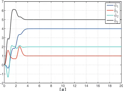
3.1. Example 1: A simple example 79
Let be the signals(t) =4 cos(t) +sin(t) +2 cos(2t) +5 sin(2t). It is obvious that the series order
80
to reproduce the signal isn=2, then the order of system (7) for the conception of the observer should
81
beN= 4. Fig.2shows the estimation of the coefficients that was performed by the observer with a
82
gainλ=8, which actually was initialized with ˆν(0) =0. The step time to perform the estimation in
83
Simulink was∆t=0.005 [s] and the used solver was ODE3.
0 2 4 6 8 10 12 14 16 18 20 −2
−1 0 1 2 3 4 5 6 7
[s]
ˆ a1 ˆb1 ˆ a2 ˆb2
Figure 2.Example 1. Estimated coefficients
84
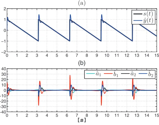
3.2. Example 2: Reconstruction of basic signals 85
This example aims to show the estimation of the coefficients for basic signals such as square and 86
sawtooth waves. The first signal to be estimated is a square wave with angular frequencyω = 1
87
[rad/s]. The observer was tuned withλ = 15. The order of the series was set n = 2, i.e. N = 4.
88
The frequency step was setω =5 [rad/s]. The step time to perform the estimation in Simulink was
89
set∆t = 0.01 [s] and the used solver was ODE3. Fig. 3shows the signal reconstruction performed
90
by the spectral observer and the estimated coefficients. Firstly, notice that the coefficients do not 91
signal, which is not enough to represent each harmonic that compose it. Even though the coefficients 93
are not constant, the signal is estimated. Notice too that all the coefficients change abruptly at each 94
discontinuity. This feature can be used for edge detection as will be seen in the next example.
0 1 2 3 4 5 6 7 8 9 10 11 12 13 14 15
−2 −1 0 1 2
(a)
0 1 2 3 4 5 6 7 8 9 10 11 12 13 14 15
−500 −300 −100 100 300 500
(b)
[s]
s(t) ˆ
y(t)
ˆ
a1
ˆ
b1
ˆ
a2
ˆ
b2
Figure 3.Example 2. (a) Square wave reconstruction and (b) Estimated coefficients
95
Both the observer and conditions that were used to reconstruct the square wave were used to 96
reconstruct the sawtooth signal shown in Fig. 4. Notice that the convergence time is less than one
97
second and the coefficients become greater at the discontinuities.
0 1 2 3 4 5 6 7 8 9 10 11 12 13 14 15
−2 −1 0 1 2
(a)
0 1 2 3 4 5 6 7 8 9 10 11 12 13 14 15
−40 −30 −20 −10 0 10 20 30 40
[s]
(b)
s(t) ˆ
y(t)
ˆ
a1 ˆb1 ˆa2 ˆb2
Figure 4.Example 2. (a) Triangular wave reconstruction and (b) Estimated coefficients
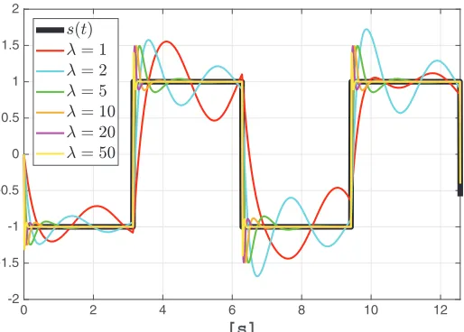
98
To end this example, we made several simulations to show how the parameterλdetermines the
99
convergence period of the estimation. Fig.5shows the estimation of the square signal when different
100
values ofλ. Notice that the bigger its value the faster it is the convergence.
0 2 4 6 8 10 12 [s]
-2 -1.5 -1 -0.5 0 0.5 1 1.5 2
Figure 5.Variations of parameterλ
3.3. Example 3: Edge detection by using the Fourier coefficients 102
Edge detection and the detection of discontinuities are important in many fields. In image 103
processing, for example, one often needs to determine the boundaries of the items of which a 104
picture is composed, [12] or in applications that utilizes time-domain reflectometry (TDR), which
105
is a measurement technique used to determine the characteristics of transmission lines by observing 106
reflected waveforms. TDR analysis begins with the propagation of a step or impulse of energy into 107
a system and the subsequent observation of the energy reflected by the system. By analyzing the 108
magnitude, duration and shape of the reflected waveform, the nature of the transmission system 109
can be determined. TDR is a common method used to localize faults in transmission lines —such a 110
leaks in pipelines or faults with small impedance in wires— because faults in transmission lines cause 111
discontinuities in the reflected waveforms. For this reason, methodologies to detect discontinuities 112
are required in order to localize the nature and position of the faults. 113
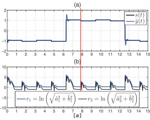
In order to shows how the spectral observer (13) can be used to detect discontinuities
in a function, we present the following example: Let us consider s(t) = sign(sin(0.5t))−
0.05sign(sin(2t)), which is plot in Fig. 6(a). The aim of this test is to detect the discontinuities in
the principal signal with periodT=2 [s]. To identify the discontinuities, the coefficients provided by
the spectral observer are used to calculate the following indicator function:
rk =ln q
ˆ a2
k+bˆ2k
(15)
The observer to perform the estimation was tuned withλ=15. The order of the series was setn=2,
114
i.e. N = 4. The frequency step was setω = 1 [rad/s]. The step time to perform the estimation in
115
Simulink was set∆t=0.01 [s] and the used solver was ODE3.
116
Fig. 6(a) showss(t)and its reconstruction ˆy(t). Fig6(b) shows the indexr1(t)andr2(t)that
117
becomes greater at the discontinuities indicating where they are. 118
3.4. Example 4: Fitting complex signal: the Bitcoin price 119
Bitcoin is the longest running and best known cryptocurrency in the world. It was released 120
as open source in 2009 by the anonymous Satoshi Nakamoto. Bitcoin serves as a decentralized 121
medium of digital exchange, with transactions verified and recorded in a public distributed 122
0 1 2 3 4 5 6 7 8 9 10 11 12 13 14 15 −2
−1 0 1 2
(a)
0 1 2 3 4 5 6 7 8 9 10 11 12 13 14 15
−10 −5 0 5 10
(b)
[s]
s(t) ˆ
y(t)
r1= ln
3q
ˆ
a2 1+ ˆb21
4
r2= ln
3q
ˆ
a2 2+ ˆb22
4
Figure 6.Example 3. (a) Signal reconstruction and (b) Estimated coefficients
intermediary. Hereafter, we will use the proposed spectral observer for fitting the historical
124
Bitcoin market close data every 1000 [min]. The records were downloaded from the website:
125
https://www.kaggle.com/neelneelpurk/bitcoin/data. 126
0 200 400 600 800 1000 1200 1400 1577
0 0.2 0.4 0.6 0.8 1 1.2 1.4 1.6 1.8
2x 10 4
samples
USD
Bitcoin Bitcoin estimation
Figure 7.Example 4. Bitcoin fitting
The observer to perform the estimation was tuned withλ = 1. The order of the series was set
127
n = 20, i.e. N = 40. The frequency step was setω = 10 [rad/s]. The step time to perform the
128
estimation in Simulink was set∆t=0.01 [s] and the used solver was ODE8.
129
In Fig. 7, the Bitcoin fitting performed by the spectral observer is shown. Fig. 8 shows
130
the estimated coefficients which are not constant and look as they were enveloped by exponential 131
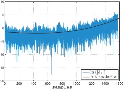
functions. In order to have a model that represents the behavior of the Bitcoin in the specified interval, 132
we can fit each coefficients by means of polynomials after calculating the natural logarithm of each 133
one. In Fig.9, ln(|a1|)is plotted versus a cubic polynomial calculated to interpolate it.
134
We can perform the same procedure for each coefficient to obtain a series with the following 135
form: 136
ˆ
y(t) =e|(αc1t3+βc1t2+γc1t+δc1)|cos(ωt) +e|(αs1t3+βs1t2+γs1t+δs1)|sin(ωt)
+e|(αc2t3+βc2t2+γc2t+δc2)|cos(2ωt) +e|(αs2t3+βs2t2+γs2t+δs2)|sin(2ωt) (17)
+...+e|(αcnt3+βcnt2+γcnt+δcn)|cos(nωt) +e|(αsnt3+βsnt2+γsnt+δsn)|sin(nωt)
whereαck,βck,γck,δck,αsk,βsk,γsk,δskare the coefficients of the polynomial that approximates the
137
natural logarithms of the coefficients. 138
0 200 400 600 800 1000 1200 1400 1577
−500 −300 −100 100 300 500
samples
Figure 8.Example 4. Estimated coefficients
0 200 400 600 800 1000 1200 1400 1600 −20
−15 −10 −5 0 5 10
samples
ln (|ˆa1|) Interpolation
Figure 9.Example 4. log|a1|vs. interpolation
3.5. Example 5: Estimation of the input force on a Duffing oscillator 139
One of the advantages of the proposed spectral observer is its structure, which is a chain of 140
integrators expressed in state-space representation. Such a structure permits to couple the observer 141
estimation purposes. With this in mind, we present an example to show how the spectral observer 143
can be coupled to the model of a given system, even with nonlinear structure such as the Duffing 144
oscillator, in order to estimate an exogenous input affecting its behavior. 145
The Duffing oscillator is expressed by the following equation:
¨
x(t) +δx˙(t) +αx(t) +βx3(t) =u(t) (18)
wherex(t)is the displacement, which is assumed as available in this example, ˙x(t)is the velocity and
146 ¨
x(t)is the acceleration. In addition, δ,αandβare parameters, which in this example are assumed
147
to be known. Finally,u(t)is an external force, which is unknown and can be estimated by using our
148
proposed observer. To achieve this goal, the following steps need to be executed. 149
Step 1. Eq. (18) must be set in state-space representation. To execute this step, we definex1(t) =
x(t)andx2(t) =x˙(t)as the state variables, such that we obtain the following equation system:
˙
x1(t) =x2(t),
˙
x2(t) =−δx2(t)−αx(t)−βx3(t) +u(t), (19)
y(t) =x1(t).
If the Liénard transform [13] is applied to system (18) in order to set it in a more appropriate form for
estimation purposes [14], it becomes
˙
x1(t) =x2(t)−δx1(t),
˙
x2(t) =−αx1(t)−βx31(t) +u(t), (20)
Step 2. Sinceu(t)is unknown and needs to be estimated, we propose its estimation by using a spectral
observer withn=1. Therefore, we coupled in cascade equation system (18) with equation system (4)
as follows:
˙
x1(t) =x2(t)−δx1(t),
˙
x2(t) =−αx1(t)−βx31(t) +ν1(t), (21)
˙
ν1(t) =ν2(t),
˙
ν2(t) =−ω2ν1(t),
y(t) =x1(t),
whereν1(t) =u(t), i.e. it is the force to be estimated.
150
System (21) can be set in the following form:
˙ x1(t)
˙ x2(t)
˙ ν1(t)
˙ ν2(t)
| {z }
˙ ξ(t)
=
0 1 0 0
0 0 1 0
0 0 0 1
0 0 −ω2 0
| {z }
A
x1(t)
x2(t)
ν1(t)
ν2(t)
| {z }
ξ(t)
+
−δy(t)
−αy(t)−βy3(t)
0 0 ,
| {z }
ϕ(ξ(t))
(22)
y(t) = [1 0 0 0]ξ(t) =Cξ(t) =x1(t), (23)
which according to [15] is uniformly observable. Therefore, a state observer expressed as ˆ˙ξ(t) =
151
Aξ(ˆt) +ϕ(ξ(ˆt)) +K(x1(t)−ξˆ1(t))can be designed for system (22), whereK can be calculated by
152
means of Eq. (14).
153
For the simulation, the paramaters of the Duffing oscillator were set: α = 1, β = 1 andδ =
154
0.3; and their initial conditions were setx(0) = [−1 −5]. The force applied to the oscillator was
155
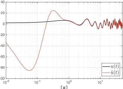
u(t) =2 cos(2t) +5 sin(2t) +4 sin(0.5t). The observer was tuned withλ = 10,ω = 1 [rad/s] and
their initial conditions were fixed as ˆξ(0) = [0 0 0 0]. Finally, the used solver was ODE 3 with a step 157
time ∆t = 0.01 [s]. The results of the estimation is shown in Fig. 10, which particulary presents a
158
comparison between the force and its estimation. Notice that the estimation converges to the force in 159
1 [s]. 160
10-2 10-1 100 101
[s] -100
-80 -60 -40 -20 0 20 40
Figure 10.Example 5. Force estimation
4. Comparative analysis vis-à-vis the STFT 161
A spectral observer can be used to determine the frequency content of local sections of a signal as it changes over time. The classic technique for performing this task is the Short Time Fourier Transform, which is the Fourier Transform with a suitable chosen windowing function. Ensuing, we present an example to compare the results of using the STFT with the results provided by the spectral
observer. For this purpose, we used the MATLABc codes created by Hristo Zhivomirov to compute
STFT and its inverse [16]. The signal analyzed was
s(t) =
0 0≤t<100[s]
sin(10πt) 0≤t<300[s]
0 300≤t<400[s]
sin(4πt) 400≤t<600[s]
0 600≤t<700[s]
(24)
sampled at 1000 [Hz]. To compute the STFT by using the code of Zhivomirov, the following
parameters were set: τw = 28[s] as the window length,h =τw/4 [s] as the hop size andnf f t = 210
as the number of FFT points. The tuning of the spectral observer was done by settingn =10,λ=1,
ω = π[rad/s] and ˆν(0) = 0. The solver used for the numerical solution was ODE4 (Runge-Kutta)
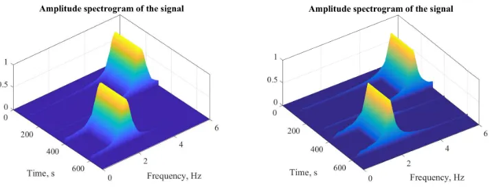
with a fixed step size∆t=0.01 [s]. The spectrograms that were produced by the STFT and the spectral
observer, respectively, are presented in Fig.11. To construct the observer spectrogram, we computed
de magnitude of each harmonic by means of the following equation:
|Ak|= p
ak+bk. (25)
On the one hand, sincen=10, the resulting vector containing the magnitude of each harmonic
162
was A= [A1 A2 A3 A4 A5 A6 A7 A8 A9 A10]. On the other hand, since the angular frequency step
163
was chosenω =π[rad/s], the resulting frequency vector was f = [0.5 1 1.5 2 2.5 3 3.5 4 4.5 5][Hz].
164
Then, the spectrogram resulted of plotting f versusA.
165
Notice that the spectrogram generated by using the spectral observer presents a better frequency 166
resolution with respect to the spectral observer. This fact can be better appreciated in Fig. 12.
However, this does not mean that the observer’s performance is superior, since it is well known that 168
the frequency resolution can be improved by widening the time window length of the STFT, even 169
if this widening implies a decreasing of the time resolution. In the case of the spectral observer, the 170
frequency resolution is adjusted by manipulating the parameterλ.
171
Figure 11.(a) STFT spectrogram (b) Spectral observer spectrogram
Figure 12.(a) STFT spectrogram (b) Spectral observer spectrogram
It is necessary to point out here that both the frequency resolution and the time resolution do not 172
only depend on the parametersτandλ, also the parametershynf f tused in the STFT algorithm and
173
ωandnused in the spectral observer, play an important factor; nevertheless, the adjustment of these
174
parameters directly affects in the computational burden and the amount of data to be processed. 175
5. Results and discussion 176
We have introduced an algorithm to reconstruct signals at the same time that their frequency 177
components are calculated: a new spectral observer. In order to show its applicability, we have 178
presented some examples, which in addition, have allowed us to glimpse some advantages and 179
disadvantages of its use. Firstly, we found the following benefits: (1) The structure of the observer, 180
as a chain of integrators, is very adequate for control and parameter estimation purposes. (2) The 181
signal is progressively incorporated at each iteration. (3) The operations required for the observer 182
implementation are with real numbers, which simplifies its programming in single-board computers. 183
(4) The gain of the observer can be easily computed by means of a simple numerical algorithm. (5) The 184
convergence of the observer is exponential, this means that the convergence period can be adjusted 185
by means of a unique parameter λ, which is a clear advantage with respect to other well-known
186
algorithms such as the proposed in [17], where the convergence period cannot be manipulated by a
unique parameter. However, there are some drawbacks that we have found for the proposed observer. 188
(1) The computational cost can be high for a small frequency resolution. (2) The algorithm must be 189
complemented with a methodology to chooseωandλin order to obtain the best estimation.
190
To conclude the discussion, it is necessary to emphasize that the spectral observer is an algorithm 191
that, like the STFT, can be used to perform a frequency-time analysis of a frequency varying signal 192
by computing the Fourier Transform (FT) during time intervals. However, there are some differences 193
to remark. (a) The STFT requires operations with complex numbers, the spectral observer does not. 194
(b) The spectral observer computes the FT and its inverse at the same time, which is a clear bonus, 195
because in case of using a recursive STFT we only get the FT, if we want to recover the reconstructed 196
signal, we must compute the Inverse Short Fourier Transform. 197
6. Conclusions 198
In this paper, we presented the design of a novel spectral observer, which can be used to 199
approximate periodical and non-periodical signals via state estimation. To design the spectral
200
observer, we constructed a synthetic system in state space representation from the Fourier series. 201
We presented some application examples to reconstruct periodical signals but also a well-know 202
non-periodical one such as the price of the Bitcoin from its genesis. Some important aspects were 203
not discussed in this article that require a deeper analysis, such as a comparison between the 204
computational burden of the spectral observer and that of the Fourier transform or an analysis of the 205
spectral observer vis-à-vis perturbations and noise. These aspects must be treated in a continuation 206
of this research work. 207
Author Contributions: Lizeth Torres conceived the spectral observer presented in this article. Javier 208
Jiménez-Cabas and José Francisco Gómez-Aguilar conceived, designed and performed the simulation tests. 209
Pablo Pérez-Alcazar advised the rest of the authors. All the authors wrote the paper. 210
Conflicts of Interest:“The authors declare no conflict of interest.” 211
Appendix MATLAB CODES 212
Appendix A.1 Symbolic computation of matrix Aω
213
syms w t 214
n=10; %Order of the Fourier Series 215
for k=1:2*n; 216
Aw(k,k)=((-1)^((mod(k-1,4)-mod(k-1,2))/2))*w^(k-1); 217
end 218
Appendix A.2 Symbolic computation of matrix Aω
219
syms w t 220
n=10; %Order of the Fourier Series 221
for k=1:n 222
for m=1:n 223
Ak(2*m-1,2*k-1)=k^(2*m-2); 224
Ak(2*m,2*k)=k^(2*m-1); 225
end 226
end 227
Appendix A.3 Symbolic computation of matrixΩ
228
syms w t 229
n=10; %Order of the Fourier Series 230
O(1,(2*k)-1)=os(k*w*t); 233
O(1,(2*k))=sin(k*w*t); 234
O(m,(2*k)-1)=diff(O(m-1,2*k-1),'t'); 235
O(m,(2*k))=diff(O(m-1,2*k),'t'); 236
end 237
end 238
239
1. Hostetter, G.H. Recursive discrete Fourier transformation. IEEE Transactions on Acoustics, Speech and 240
Signal Processing1980,28, 184–190. 241
2. Bitmead, R.R.; Tsoi, A.C.; Parker, P.J. A Kalman filtering approach to short-time Fourier analysis. IEEE 242
Transactions on Acoustics, Speech and Signal Processing1986,34, 1493–1501. 243
3. Orosz, G.; Sujbert, L.; Peceli, G. Spectral observer with reduced information demand. Instrumentation 244
and Measurement Technology Conference Proceedings. IEEE, 2008, pp. 2155–2160. 245
4. Na, J.; Yang, J.; Wu, X.; Guo, Y. Robust adaptive parameter estimation of sinusoidal signals. Automatica 246
2015,53, 376–384. 247
5. Bitmead, R.R. On recursive discrete Fourier transformation. IEEE Transactions on Acoustics, Speech and 248
Signal Processing1982,30, 319–322. 249
6. Torres, L.; Gómez-Aguilar, J.; Jiménez, J.; Mendoza, E.; López-Estrada, F.; Escobar-Jiménez, R. Parameter 250
identification of periodical signals: Application to measurement and analysis of ocean wave forces.Digital 251
Signal Processing2017. 252
7. Dash, P.K.; Khincha, H. New algorithms for computer relaying for power transmission lines. Electric 253
Machines & Power Systems1988,14, 163–178. 254
8. Houmb, O.; Overvik, T. Some applications of maximum entropy spectral estimation to ocean waves and 255
linear systems response in waves. Applied Ocean Research1981,3, 154–162. 256
9. Blödt, M.; Chabert, M.; Regnier, J.; Faucher, J. Mechanical load fault detection in induction motors by 257
stator current time-frequency analysis.IEEE Transactions on Industry Applications2006,42, 1454–1463. 258
10. Benbouzid, M.E.H.; Vieira, M.; Theys, C. Induction motors’ faults detection and localization using stator 259
current advanced signal processing techniques. IEEE Transactions on Power Electronics1999,14, 14–22. 260
11. Busawon, K.; Farza, M.; Hammouri, H. A simple observer for a class of nonlinear systems. Applied 261
Mathematics Letters1998,11, 27 – 31. 262
12. Engelberg, S. Edge detection using Fourier coefficients.American Mathematical Monthly2008,115, 499–513. 263
13. Liénard, A.Etude des oscillations entretenues; Revue générale de l’électricité, 1928. 264
14. Torres, L.; Verde, C.; Vázquez-Hernández, O. Parameter identification of marine risers using Kalman-like 265
observers.Ocean Engineering2015,93, 84–97. 266
15. Hammouri, H. Uniform observability and observer synthesis. InNonlinear observers and applications; 267
Springer, 2007; pp. 35–70. 268
16. Zhivomirov, H. Short-Time Fourier Transformation (STFT) with Matlab Implementation. MathWorks 269
Website, 2017. 270
17. Kušljevi´c, M.D.; Tomi´c, J.J. Multiple-resonator-based power system Taylor-Fourier harmonic analysis. 271
IEEE Transactions on Instrumentation and Measurement2015,64, 554–563. 272
273
274