CM55: special prime-field elliptic curves almost optimizing
den Boer’s reduction between Diffie–Hellman and discrete logs
Daniel R. L. Brown∗ February 24, 2015
Abstract
Using the Pohlig–Hellman algorithm, den Boer reduced the discrete logarithm prob-lem to the Diffie–Hellman probprob-lem in groups of an order whose prime factors were each one plus a smooth number. This report reviews some related general conjectural lower bounds on the Diffie–Hellman problem in elliptic curve groups that relax the smoothness condition into a more commonly true condition.
This report focuses on some elliptic curve parameters defined over a prime field size of size 9 + 55×2288, whose special form may provide some efficiency advantages over random fields of similar sizes. The curve has a point of Proth prime order 1 + 55×2286, which helps to nearly optimize the den Boer reduction. This curve is constructed using the CM method. It has cofactor 4, trace 6, and fundamental discriminant−55.
This report also tries to consolidate the variety of ways of deciding between elliptic curves (or other algorithms) given the efficiency and security of each.
Contents
1 Introduction 3
2 Previous Work and Motivation 4
2.1 den Boer’s Reduction between DHP and DLP . . . 4
2.2 Complex Multiplication Method of Generating Elliptic Curves . . . 4
2.3 Earlier Publication of the CM55 Parameters . . . 4
3 Provable Security: Reducing DLP to DHP 5
3.1 A Special Case of den Boer’s Algorithm . . . 5
3.2 More Costly Reductions with Fewer Oracle Calls . . . 7
3.3 Relaxing the Smoothness Requirements . . . 11
4 Resisting Other Attacks on CM55 (if Trusted) 13
4.1 Resistance to the MOV Attack . . . 13
4.2 Resistance to the SASS Attack . . . 13
4.3 Risk of Low Magnitude Discriminant . . . 13
∗
4.4 Risk of Low Magnitude Trace . . . 14
4.5 Weak q-Strong DH Assumption . . . 14
4.6 Strong Static DHP . . . 14
5 Rarity and Absence of Malice 15 5.1 Malicious Algorithm Promotion . . . 15
5.2 Suspicions About the “Verifiably Random” NIST Curves . . . 16
5.3 Rarity and Other Arguments . . . 17
5.3.1 Rarity Sets: Informal Definition . . . 17
5.3.2 Formalizing Secret Attacks . . . 19
5.3.3 Uncorrelated Secret Attacks . . . 19
5.3.4 Equivalence Argument . . . 20
5.3.5 Rarity Argument . . . 20
5.3.6 Exhaustion Argument . . . 21
5.4 Rarity Sets for CM55 . . . 22
5.4.1 A First Rarity Set . . . 22
5.4.2 A Low Discriminant Rarity Set . . . 23
5.4.3 Loose Number-Theoretic Rarity Set . . . 24
5.4.4 A Rarity Set Based on Special Field and Special Curve Size . . . 24
5.4.5 Heuristics in the Rarity Sets Above . . . 25
5.5 Bad and Rare Curves . . . 25
5.6 How the CM55 Parameters were Found . . . 30
5.7 Special Curves: Serpentine Readiness and Diversity . . . 30
6 Conclusions and Questions 32 A Actual CM55 Curves 32 B Comparing Curves of Given Security and Efficiency 33 B.1 Absolute Metrics . . . 33
B.2 Excluding Defective Algorithms . . . 34
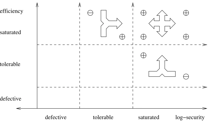
B.3 Dominance: A Partial Ordering via Metrics . . . 34
B.4 Saturated Security? Optimize Efficiency! . . . 35
B.5 Saturated Efficiency? Optimize Security! . . . 37
B.6 Trading Efficiency for Security, and Vice Versa . . . 38
B.7 Work Ratio: Security times Efficiency . . . 39
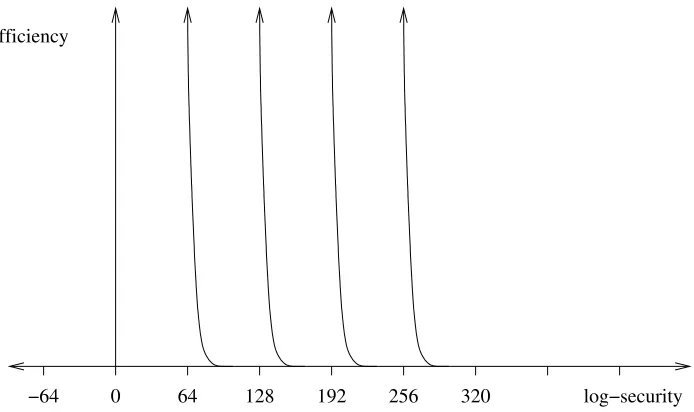
B.8 Progressive Ratio: Log-Security times Efficiency . . . 41
B.9 Curve Availability . . . 43
C Implementation Sketch 46 C.1 General Expectations . . . 46
C.2 A Naive Field Implementation Outline . . . 46
C.2.1 Big Integer Arithmetic . . . 47
C.2.2 Modular Representation and Reduction . . . 48
C.2.3 Lengthier Field Operations . . . 50
C.3 GLV and Endomorphism . . . 52
D Primality Proofs 54
E Miscellaneous Additional Data 55
1
Introduction
An elliptic curve, defined over a prime fieldFp of size 9+55×2288 and having a (Fp-rational) point with order 1 + 55×2286, which is a Proth prime, can be constructed using the complex
multiplication method. The potential benefits of these special curve parameters (CM55) are:
• it makes den Boer’s reduction [dB90] between the DLP and DHP almost as tight as possible (even if the DLP becomes weaker than expected);
• the special form of the underlying field may permit more efficient field arithmetic than for average random prime field of similar size;
• the complex multiplication properties of the curve might make the Gallant–Lambert– Vanstone method [GLV01] useful; and
• heuristic rarity properties of the curve possibly reduce the risk of some types of ma-licious curve selection attacks.
Some potential security risks of the CM55 curve parameters are:
• the significantly lower than average magnitude of its discriminant;
• the significantly lower than average magnitude of its trace;
• the special form of its field;
• larger size than usually deemed sufficient for security (usually 256 bits), with a result-ing waste of data transmission and computation;
• possible non-optimally efficient field of the given size, with a resulting waste of com-putation; and
• a possible vulnerability to an unpublished attack that affects only a rare class of curves including this curve.
This report states a theorem which adjusts den Boer’s algorithm in such a way to plausibly drop a smoothness condition making it applicable to most elliptic curve groups.
2
Previous Work and Motivation
2.1 den Boer’s Reduction between DHP and DLP
At CRYPTO 88, den Boer [dB90] proved that, in certain groups, solving the Diffie–Hellman problem (DHP) is almost as hard solving the discrete logarithm problem (DLP) by giving a reduction algorithm that solves the DLP using an oracle for solving the DHP. Specifically, if a group has a hard discrete logarithm problem and a prime ordernsuch thatn−1 is smooth, then den Boer’s reduction proves that the group has a hard Diffie–Hellman problem, which is necessary for the security of many key agreement schemes, and some other cryptographic schemes.
2.2 Complex Multiplication Method of Generating Elliptic Curves
Atkin and Morain [AM93] introduced the complex multiplication (CM) method for gen-erating elliptic curves of a given order n. It is straightforward to apply the CM method to optimize den Boer’s reduction by starting with n such that n−1 is quite smooth. To elaborate, setn= 1+swheresis smooth, then apply the CM method to find the curve over the prime field. If applied naively, the CM method results in a curve whose defining field size has the form p =n+r wherer is some random-looking integer with |r|with bit-size similar the √n, under the heuristic that Cornacchia’s algorithm provides random-looking solutions. Therefore, the two main deficiencies of this naive application of the CM method to den Boer’s work are the following.
• It results in an elliptic curve with discriminant of lower magnitude than is typical for a random elliptic curve, which is deemed a potential risk of having a easier than usual discrete logarithm problem.
• It results in a field size will have its least significant half of binary expansion essentially random, which is potentially less efficient than is possible for specially selected fields of similar size.
The CM55 curve parameters described in this paper are an attempt to somewhat resolve this latter deficiency.
Remark 2.1.Potentially, field efficiency helps the adversary as much as the user, so to some ex-tent field inefficiency may not be the deficiency it is conventionally deemed. (See §B.7 for further discussion.)
2.3 Earlier Publication of the CM55 Parameters
The CM55 curve parameters were described in patent of Brown, Gallant and Vanstone [BGV07], which also mentioned the benefit of improving den Boer’s reduction and the benefit of having a field of special size.
3
Provable Security: Reducing DLP to DHP
In this section, some variants of the den Boer reduction algorithm are stated and proven. These algorithms solve the ECDLP using an oracle for the ECDHP. These reductions show that a hard ECDLP suffices to avoid direct attacks on the ECDHP.
In particular, the reductions rule out the possibility that ECDHP is easy, or at least feasible, while the ECDLP is still hard. Although the possibility of such a gap appears unlikely, a similar-sized gap between the decision DHP and the computational DHP is known to exist for certain groups, including elliptic curve groups with low enough embedding degrees.
Remark 3.1.Some cryptographic schemes, such as many signature schemes including ECDSA, are not known to depend directly on the hardness of the ECDHP. In particular, in an ECDSA-only system, the CM55 curve has little advantage over other curves. (Some alternative signature schemes, such as the Goh–Jarecki signature scheme [GJ03], are related to the ECDHP. So, CM55 may provide some advantages to these alternative signature schemes.)
3.1 A Special Case of den Boer’s Algorithm
The following theorem is essentially a special case of a theorem due to den Boer. It makes a positive use of the algorithm first described by Pohlig and Hellman. It turns this PH attack algorithm for solving the discrete logarithm into a reduction between two conjecturally hard problems.
As in den Boer’s theorem, we are trying to keep two things low: (1) the number of calls to the DH oracle; and (2) the amount of computation in the algorithm. In den Boer’s original theorem the benefit of the second objective helps to avoid making any assumptions about the cost of the discrete logarithm problem, which may make sense in the finite field setting, where index calculus algorithm show promise for improvement.
In the elliptic curve setting, the second objective has a less likely benefit: in the event the discrete logarithm problem becomes significantly easier, but still intractable, the second objective ensures that the theorem is still applicable.
This report next restates and reproves the den Boer theorem, making it specific to the CM55 group order.
Theorem 3.1 (den Boer, special case).Suppose that G is a group of prime order n = 1 + 55×2286, and g is a generator of the group, and multiplicative notation is used for the group operation. Consider the function M : G×G → G : (gx, gy) 7→ gxy, which outputs Diffie–Hellman shared secrets, and the function L : G → Zn : gz 7→ z, which outputs discrete logarithms. Then there exists an efficient algorithm A (described in the proof) that computes functionL using at most:
• 286 calls to the function M,
• 341 calls to each of the following operations:
– an exponentiation in the group G,
– an exponentiation modulo n,
– a Chinese remainder theorem (CRT) calculation modulon−1.
Proof. Algorithm Areceives input gz and needs to computeL(gz) =z. Let us use the fact that 3 is a primitive element of the field of integers modulon. Ifgz= 1, which Acan easily detect, then z = 0. Otherwise, z 6= 0, and z = 3y modn for some y whose value matters only modulo n−1. Write:
y≡(x, w) mod (2286,55) (1) which are the CRT coordinates of y. We will use such CRT coordinates for other values. We will have 0≤w <55 andx=x0+x12 +. . . x2852285withxj ∈ {0,1}. Clearly, it suffices to find x andw, since that determinesy, and thenz.
Leth0 =gz, which is the input toL, and lethj =M(hj−1, hj−1) for 1≤j≤286, which
requires 286 applications of the functionM. Note that:
hj =gz
2j
=g3y×2
j
=g3(2j x,2j w) (2)
Computation of thesehj uses all the calls available toA. The rest of the work can only use the normal multiplication in the groupG, which corresponds to addition of thegexponents.
Compute the values:
ki =g3
2286×i
=g3(0,2286i) (3) for 0 ≤i < 55. Note that these values do not depend onz and can be pre-computed. It follows that
h286=kw (4)
So the secret w can be determined by the index w of the value kw in the list of values ki that matches h286.
Our next goal is to determine x, which we will do one bit at a time. Ifx0= 0, then
h285 =g3
(0,2285w)
. (5)
Since we know w, we can compute the value on the right using CRT, modular exponen-tiation, and the square-and-multiply algorithm for exponentiation in the group G. When we compute this value, if it matchesh285, then we conclude x0= 0, otherwise we conclude
x0 = 1. In either case, we have determined x0. Next, we test ifx1= 0 by computing if
h284 =g3
(2284x0,2284w)
. (6)
Again we can compute the right hand side conventionally. The boolean truth value of (6) matches the boolean truth value of the equation x1 = 0. So we can determinex0. We find
x2, by using x0,x1 and h283. Keep iterating in the same manner to find all the bitsxj. Note that in addition to the 286 calls to M, algorithm Adoes about 55 + 286 = 341 of each of the following operations:
• a CRT calculation forn−1,
• an exponentiation modulo n−1,
• an exponentiation in the group G
which is what the theorem claims forA.
The immediate consequence of Theorem 3.1 is that the cost of the ECDHP is at least 286−1 ≈ 2−8.26 times the cost of the ECDLP, approximately, almost regardless of how difficult the ECDLP is. More precisely, this lower bound on the ECDHP holds provided that the cost of the ECDLP dominates the cost of the reduction (the 341 calls to the four operations listed in the theorem). In the next section, we consider the interplay between higher-cost reductions and assumptions of a higher cost for the ECDLP.
Note that the algorithm we used above is simpler than den Boer’s original algorithm for a few reasons. First, it works over a prime order group. Second, it mainly takes advantage of one prime factor two (but repeated multiple times). Third, it treats the prime factors 5 and 11 together as a single factor of 55. Fourth, rather than using Shanks’ baby-step-giant-step (BSGS) algorithm for each factor, it just uses a table look-up.
In particular, the actual den Boer algorithm would have been more efficient in deter-mining (4), but would have used slightly more calls to M. Following den Boer’s approach of using the BSGS algorithm, we could determinekw using just 15 exponentiations instead of 55 exponentiations, as follows. For 0≤i <7 and 0≤f <8, compute the pair of values
ki=g3
(0,2286×i)
(7)
h286,f =h3
(0,2286×8f)
286 , (8)
and then find a pair (i, f) with ki =h286,f which will determine thatw =i−8f mod 55. This is only a small gain in efficiency, but in the next section, we try to extend this approach to further reduce the calls made to M. Furthermore, instead of using BSGS, we will use Pollard rho.
Remark 3.2.The fact 2286|n−1 in Theorem3.1 makes the tightness of low cost reduction nearly optimal in the sense of using the very few calls to M. In other words, the n is nearly optimal in regards to certain types of security.
Remark 3.3.Theorem 3.1 assumes a perfect DH oracle M. Previous other work, such Shoup’s [Sho97], considers the problem of handling imperfect DH oracles in such reductions. A first step in handling imperfect DH would be to blind the inputs, just in case the oracle always fails for the inputs of the kind our algorithm generates. Then some kind of error handling might apply. Future work may fill in the necessary details to adapt these techniques to the improved specific result in Theorem3.1.
3.2 More Costly Reductions with Fewer Oracle Calls
In this section, a slight variant of the den Boer reduction is described. This variant uses fewer DH oracle calls, but a greater amount of computation. By allowing the amount of computation to approach what one usually conjectures to be the cost of the discrete logarithm problem, one can minimize the number of oracle calls.
of this approach is that to apply optimally (accurately), one has to be quite (moderately) careful about the complexity of the algorithms. We will use some constants to abstract away some of this level of detail.
It will suffice for stating the theorem to describe the average running time of the Pollard rho as taking C1
√
m iterations on average in a cyclic group of size m. (Note: we will not assume thatm is prime.)
This time around, we will use additive notation in the proof. This will make it look less like den Boer’s original proof, but will make it more like the traditional elliptic curve cryptography notation, which is where we intend to apply the result. It will also make it more like Boneh and Lipton’s results [BL96] for the black-box field problem. It will also reduce the power tower notation from three levels of superscripts to two.
Theorem 3.2. LetGbe a group of prime order n= 1 + 55×2286, with additive notation and generator G. Let D be an DH oracle such thatD(aG, bG) =abG for alla, b∈Z. Let
dbe an integer with1≤d≤286. GivenA∈G, one can computez∈Zsuch thatA=zG, using dcalls toD, and at most, on average,
(286−d) +
C1
√
55×2143−d/2
(9)
calls to each of the following four operations:
• two pseudorandom functions,
• a scalar multiplication in the group G,
• an exponentiation modulo n, and
• an exponentiation modulo n−1.
Proof. To test z = 0, check if A = 0G. Otherwise, there exists an integer y, which the algorithm will try to find, such thatz= 3y modn with 0≤y < n−1 = 55×2286. Write:
y=x(2286−d×55) +w (10)
for integers x and w with 0 ≤x < 2d and 0 ≤ w < m = (n−1)/2d = 55×2286−d. The algorithm will next try solve for w using a version of the Pollard rho algorithm, and then solve forx one bit at time, using the usual Pohlig–Hellman algorithm.
Let H0 =A, and letHj =D(Hj−1, Hj−1) for 1≤j≤d, which requiresdapplications
of the DH oracleD. Note that:
Hj =z2
j
G= 3y×2jG. (11)
In particular,
Hd= 3w×2
d
G. (12)
We will try to run Pollard rho over them element set:
M={32 d×i
For this, will need two pseudorandom functions:
f :M→Zm (14)
F :M→ {G, Hd} (15)
LetR0=G. Forj≥0, let
Rj+1 = 32
d×f(R j)F(R
j) (16)
Compute and track quadruples (Rj−1Rj, R2j−1, R2j) until Rj = R2j, which we can call a Floyd collision. In the event that F(Rj−1) = F(R2j−1), which should happen with
probability about one half, start over with new pseudorandom functions f andF (perhaps changing any keys that the functions use). Eventually, we should get a Floyd collision in which F(Rj−1)6=F(R2j−1) and therefore either:
32df(Rj−1)G= 32d(f(R2j−1)+w)G; (17)
or the same withj−1 and 2j−1 swapped. But this means that either,
w≡f(Rj−1)−f(R2j−1) modm (18)
or the modular negation. The expected number of Rj that need to be computed is given by C1
√
m, in accordance with our definition of the constantC1.
Once w is determined, we proceed similarly to the proof of Theorem 3.1 to determine the bits of x, one at a time. Let x =x0+x1+· · ·+xd−12d−1. We can determine x0 by
looking at:
Hd−1 = 3(x0×2
d−1×55)+(w×2d−1)
G (19)
Since we now know w, after having applied Pollard rho, there are only two possible value of x0, one of which can pick to compute the right-hand side of the equation above. If it
matches, then we know our guess atx0is correct. Then continue by usingHd−2 to determine
x1 and so on, finishing by usingH1 to determine xd−1.
Now we take a common conjecture for elliptic curves in general, and specify it to the CM55 curve(s).
First some more details about the Pollard rho algorithm, in its conventional application to solving the ECDLP. Each iteration of the pseudorandom operation costs aboutC2 group
operations on average, amortized over the execution of the whole algorithm. I think a series work, especially by Teske [Tes01], addresses empirically and theoretically how low C2 can
go (I hope to update this report accordingly upon reviewing such research). For a concrete example, supposeC2 = 2.
Conjecture 3.3.All algorithms that solve the ECDLP over the curve CM55 cost at least the equivalent of:
C3C2C1
√
n (20)
If Pollard rho is the optimal algorithm for solving the ECDLP, then C3 = 1. But
perhaps some other algorithm is better, in which case C3 < 1. The lower bound 2−16
in the conjecture is chosen so that the ECDLP in CM55 would fare about as well as an arbitrary curve group with order approximately 2256 such that Pollard rho is the fastest ECDLP in this group. This accounts for the suspicion about low magnitude discriminant by estimating any improvement in the ECDLP due to the low discriminant produces only a 216 times speedup in the ECDLP. Of course, it is possible that the low discriminant could have a much greater effect, or even that all elliptic curves are more effected. So, the content of the conjecture is a quantified expression of confidence in the CM55 parameters. The main justification for this confidence, at a qualitative level, is that low discriminant curves have long been suspected, and even used in BitCoin, but no attack has been published. The exact quantitative level of confidence in this conjecture has been selected more for convenience of the CM55 parameters.
Remark 3.4.Gallant, Lambert and Vanstone [GLV00] showed how to speed up generic attacks on the ECDLP in groups equipped with an efficient endomorphism, specifically Koblitz subfield curves defined over a binary field. I suspect that such a speed-up relies on the endomorphism being more efficient than a group operation. In other words, it appears to me that generic group algorithms will not be helped substantially by endomorphism less efficient than a group algorithm. I expect any endomorphism of CM55 curves to be less efficient than the group operation. If CM55 is lucky, then its endomorphism will help the user more than the adversary. I hope that further research will resolve these types of uncertainties.
While writing this paper, I have begun to wonder about Silverman’s xedni calculus at-tack for solving the ECDLP, which Jacobson, Koblitz, Silverman, Stein and Teske [JKS+99] show to be infeasible in general. In particular, I wonder if the xedni attack might some-how be more effective for low discriminant elliptic curves. Recall that the xedni calculus strategy involves lifting the finite field points of the curve to rational points, and thus into the complex numbers. The CM method finds finite field curves already related to curves over the complex numbers. Perhaps this pre-existing link between the finite field curve and complex curve in the CM method can be exploited in a variant of the xedni calculus. I have no expertise in the area, but the vague argument above, plus the suspicion expressed by many others about low discriminant curves is enough to convince me to state my conjecture forC3 as low as 2−16 in the case of CM55.
Now let C4 be the average number of CM55 group operations needed to perform each
the scalar multiplication in the reduction algorithm of Theorem 3.2. We expect C4 to be
larger than C2. Again, one can amortize some of the costs, do some upfront calculations
and so on. Let us estimateC4 = 350 for the sake of a concrete example. Note that it will
turn out to be the case that the largeness of the difference between C4 and C2 affects the
tightness of the lower bound on the ECDHP.
The next step is to optimize d to gain the highest lower bound on the cost of the ECDHP based on Theorem 3.2. For the sake of simplicity, we will ignore the cost of the pseudorandom functions, and exponentiations modulo n and n−1 in the reduction algorithm. A more thorough analysis should include these costs.
operations. Then Theorem 3.2and Conjecture3.3 say that
dX+C4(286−d) +C4C1
√
55×2143−d/2 ≥C3C2C1
√
n. (21)
Fordenough smaller than 286, the termC4(286−d) will be dominated by the term to its
right by virtue of the factor 2143−d/2, so can be dropped with negligible loss of accuracy. This allows us to write a lower bound of:
X≤C3C2C1
√
n1
− C4
C3C22d/2
d (22)
To make this concrete, put (C1, C2, C3, C4) = (1,2,1,350), and try to optimized. This gives
an optimal value of d= 21, and placesX at least 0.042≈2−4.58 times the cost of Pollard rho.
The tightness of the reduction compared Theorem 3.1 has been slightly improved in the analysis above. Furthermore, because the value of d above is smaller, Theorem 3.2
can be generalized to groups of order n where n−1 is only divisible by 2d. This gain in generality is largely due to the rather strong assumption in the corresponding generalization of Conjecture 3.3to other groups.
The event of ECDLP being much more quickly solvable than Pollard rho can be rep-resented by setting C3 even smaller. For example, setting C3 = 2−30, which is below the
estimate in the conjecture, the optimaldseems to be 87, and the tightness of the reduction is 2−6.5. Again, Theorem3.2should generalize to n−1 having a factor of 287. For smaller
C3, one will get larger d, and one has to be more precise with the estimates to ensure
accuracy.
3.3 Relaxing the Smoothness Requirements
In this section, we state a version of den Boer’s theorem that does not rely on any smoothness conditions. Instead, it relies on the existence of a factor of a certain size, similar to the Brown–Gallant (BG) algorithm [BG04] (which Cheon [Che10] extended). Indeed, in some sense, it is an application of the BG algorithm because a full DH oracle can of course be used to implement the static DH oracle used in the BG algorithm. The main difference is the algorithm here uses fewer oracle calls, because a full DH oracle is available, not just a static DH oracle.
Theorem 3.4. Let G be a group of prime order n = 1 +uv, with additive notation and generator G. LetD be an DH oracle such thatD(aG, bG) =abGfor all a, b∈Z. Given A one can computez∈Z such thatA=zG, using at most 2 log2(u) calls toD, and at most, on average,2√v+ 2√u calls to each of the following four operations:
• a scalar multiplication in the group G,
• an exponentiation modulo n, and
• an exponentiation modulo n−1.
by avoiding the constantC1, and instead of computingHd= 3w×2
d
Gby usingdcalls toD, effective applyingdsquaring operations to the logarithm, we instead a square-and-multiply strategy to compute H = 3wuG. (Again, z = 3y modn and y =xv+w where 0 ≤x < u
and 0≤w≤v.
We then solve for w using BSGS using about 2√v scalar multiplications and modular exponentiations. We must then solve forx, which can also be done using BSGS at a cost of 2√u scalar multiplications and modular exponentiations.
The tightness of the resulting reductions has an analysis similar to that of Theorem 3.2. The two main differences are as follows.
• There must exist a factor u of the optimal size. Small factors are likely, for random
n, but are likely a little off from optimal in size.
• Theorem 3.2 has u = 2d which minimizes the number of calls to M, thus making the reduction tighter than average, by one bit, according to Theorem3.4but perhaps improvable to only half a bit tighter.
Theorem 3.4 does not concern CM55 directly, but is useful for comparing CM55 to other curves. In particular, it shows that CM55 can achieve a tighter reduction than typical curves, but the reduction is not dramatically tighter.
Remark 3.5.When first writing about the CM55 in the patent [BGV07], I did not contemplate a result such as Theorem3.4. Consequently, I was under the mistaken belief that the CM55 parameters represented a more substantial improvement in the tightness of the reduction between the DHP and DLP.
Therefore, the main direct benefit of group orders like that of CM55 group is that they nearly optimize the tightness of these kinds of bounds over a large range of situations.
Remark 3.6.This also helps in arguing that the CM55 parameters were not selected maliciously but rather according to a principle of optimizing provable security. More precisely, if we assume that a weakness in the curve does not correlate to optimizing the den Boer reduction, then by optimizing the den Boer reduction we reduced some of the wiggle room to allow a malicious search. These issues will be discussed in further detail later in§5.
Remark 3.7.Very loosely speaking, if the ECDLP in general collapses from about√nto far enough below √4ngroup operations in difficulty, then Theorem3.4 can no longer offer much protection for
the ECDHP. Theorem 3.1 would still apply. For other curves, ECDHP might collapse further to no security, much like the ECDDHP collapses when pairings become efficient. Under these unlikely disastrous conditions, CM55 would retain about 265group operations for the security the ECDHP, which is quite low, but still out of reach for many adversaries. Perhaps there exists a curve similar to CM55, but with an extra margin of error, that can better tolerate such a collapse.
In this situation, a Maurer–Wolf reduction [MW96] would be useful. For example, the auxiliary curves of Muzereau, Smart and Vercauteren [MSV04] can be used for the NIST curves, to provided some kind of lower bound on the ECDH in the event of a √4n attack on the ECDLP. In this case,
4
Resisting Other Attacks on CM55 (if Trusted)
This section reviews well-known (suspected potential) attacks, that can affect certain elliptic curves, but can normally be avoided by an appropriate choice of elliptic curve. For each attack, this section considers its applicability to the CM55 curves.
For the purposes of assessing the risk of well-known suspected potential attacks, such as on low-magnitude discriminant curves, this section presumes either that the CM55 curve was not selected maliciously, or that its selector, that is me, was incapable of actualizing any of these potential attacks.
A skeptical reader, who is cautious about elliptic curves being maliciously promoted, yet is also in some way interested in using the CM55 curve, might seek to verify the arguments in§5 to allay some (but not all) of these concerns.
4.1 Resistance to the MOV Attack
The Menezes–Okamoto–Vanstone (MOV) attack [MOV93] solves the discrete logarithm in an elliptic curve group if the elliptic curve group has a sufficiently low embedding degree. The embedding degreeB for an order nsubgroup of an elliptic curve defined over a prime field of size p is the smallest non-negative integers such that pB ≡ 1 modn. In other words, it is the order of p modulo n. For example, if n = p + 1, then B = 2, since
p2 ≡(−1)2≡1 modn.
The MOV attack works by converting the discrete logarithm problem in the elliptic curve group into the discrete logartihm problem in an order-nsubgroup of the multiplicative group of the the finite field of sizepB. For low values ofB, the finite field problem can be solved using an index calculus algorithm, such as the finite field sieve algorithm, which is faster then generic algorithms like Pollard rho.
The CM55 curve appears to have an MOV embedding degree B = (n−1)/2, which is the second highest possible value (the next below maximal value of (n−1)). This value is well above the threshold to make MOV attack effective, which could be anywhere between 20 to 100. Indeed, even storing a random elenent of the finite field of sizae pB is infeasible, let alone running any algorithm in the field.
4.2 Resistance to the SASS Attack
The Smart–Araki–Satoh–Semaev (SASS) attack, [BSS99,§V.3] solves the discrete logarithm problem in elliptic curve groups whose size equals that of the underlying field. In other words, it affects trace one curves.
The CM55 curve has size p−5, not p, so is not affected by the SASS attack. It has trace six, not trace one.
4.3 Risk of Low Magnitude Discriminant
The discriminant is −55 which is significantly lower magnitude than it would be for a random curve.
Conjecture3.3.
Perhaps future research can find a curve with a discriminant large enough to allay these concerns, yet, like CM55, still with a tight den Boer reduction, and with an efficient underlying field.
4.4 Risk of Low Magnitude Trace
The CM55 curves all have trace 6. This is significantly lower magnitude than for random curves, with a p-value of about 2−145.
Low trace curves are not usually considered a typical risk, but this may be partly due to the relatively few proposals for low trace curves. In fact, both the MOV and SASS attacks can be described as affecting low trace curves, namely trace zero and trace one curve, respectively.
Proposing the low-trace CM55 curve in this report may prompt further investigation into low-trace curves. Perhaps the MOV and SASS attacks have a common generalization to other low-trace curves. If so, then this would be bad for CM55, but I think would improve the general understanding of ECC.
4.5 Weak q-Strong DH Assumption
The q-strong DH assumption [BB04] is optimally weak in this group. In particular, per [BG04], it is not optimal for use in cryptographic schemes that expose the raw DH secret, such as some variants of the Ford–Kaliski key retrieval scheme [FK00], and the Passmaze protocol [Bro05].
Remark 4.1.The security against the q-strong DHP is an example of security characteristic that is negatively correlated to the goal of optimizing the den Boer reduction. Any user considering whether or not to trust CM55, must not only be careful not to rely on theq-strong DHP, but must assess the risk that some other attack correlates negatively the tightness of the den Boer reduction.
4.6 Strong Static DHP
The static Diffie–Hellman Problem, formalized by Brown and Gallant [BG04], like the ordinary DHP, becomes harder for CM55 in the sense of having a tighter reduction. This is an example of a positive correlation between two security properties.
Unlike the q-strong DHP, most ECDH-based protocols rely to a degree on the static DHP to be hard: namely, any protocols that allow re-use of ECDH private keys. Of course, such protocols can just rely on the ordinary DHP too, but only if they assume perfect key generation. Given the many examples of poor key generation in deployed products discovered by Lenstra’s team [LHA+12], the assumption of perfect key generation seems a little too strong. If static DH keys are biased but still unguessable, then the security appears to rely on the static DHP being hard.
the value of this reduction is in reducing the threat that some other kind of weak keys have to be avoided for static ECDH problem.
To justify why weak keys might be a greater threat for ECDHP than for ECDLP, consider the case of the ephemeral keys used in ECDSA and Schnorr signatures. These suffer from weak key generation attacks, where the weakness is very mild and has nearly no impact on the ECDLP. In other words, there is a large gap between in the conditions for secure key generation in the context of imperfect key generation. In particular, there is no reduction between the hardness of the problems under weak key generation settings. (Just to be clear, some security proofs for these signatures would assume perfect key generation.) If these weak key generation for ElGamal-based signature had remained unpublished, then perhaps some implementations would have taken some liberties, say for efficiency’s sake, with the generation of ephemeral secret keys in signatures, and thereby would have been vulnerable to an attack. In other words, these weaknesses would have been unforeseen.
In this light, the Brown–Gallant reduction between the static DHP and DLP, helps to ensure that that there is no such gap, and helps to assure one that the current practices in key generation are sufficient, and there are no unforeseen gaps. Maybe nobody foresees such a gap, and maybe our foresight is good enough. The CM55 curves nearly optimize this reduction, so benefit well from this security analysis.
Of course, the first line of defense against weak key generation is strong key generation. In particular, the kind of bias of question is almost certainly avoided by merely using a proper pseudorandom function. Therefore, this kind of reduction merely provides a second line of defense. Put another way, a corrupted implementation, or fault injection attack, cannot just flip a bit of the private key to defeat the security of ECDH. (By contrast, this might work against a signature scheme, or one-time pad). Put yet another way, rather than relying on the full-fledged pseudorandomness of the key generation, one can instead rely on the more modest, and hence more plausible, properties that ensure that keys do not the ECDLP weaker. In particular, for resisting known attacks, this means that the keys need to be unguessable, and to not have a sufficient bias to make the Pollard kangaroo algorithm significantly faster than Pollard rho.
5
Rarity and Absence of Malice
This section is preliminary, hypothetical and speculative, so may contain inaccuracies.
5.1 Malicious Algorithm Promotion
Various mailing list emails, web sites, and journals have cast suspicion against various NIST cryptographic standards. These suspicions postulate that the cryptographic algorithms have been maliciously promoted. In other words, NIST or its partners knew, it is alleged, of attack against these curves, yet promoted them anyway (presumably: with the belief that others will not discover the secret attacks, or else that they possess a secret key providing exclusive access to the attack; and apparently, with a lack concern about suspicions such as these.)
algorithms. In their role as NUMS numbers, these special values serve as a mechanism to persuade users that the values have not been chosen maliciously. For example, the MD5 algorithm includes constants derived from values of the sine function evaluated at integer radian values. Sometimes, these special values serve a second purpose, which is to be random-looking, in the hope to reduce the risk that some special non-random pattern might render the algorithm insecure.
5.2 Suspicions About the “Verifiably Random” NIST Curves
Some of these suspicions about NIST have been directed towards the ten “verifiably random” the NIST recommended curves [NIS99, NIS05]. Indeed, these curves do not comply with the usual nothing-up-my-sleeve approach. These curves are derived from the output of a pseudorandom function applied to a seed value. Unfortunately, the seed values look completely random and have yet to be unexplained. In particular, there is no way to confirm that the seed has not been selected maliciously. Therefore, the way the curves have been promoted does not provide any kind of NUMS effect.
Remark 5.1.Of course, the label “verifiably random” is a slight misnomer (one of many in cryptog-raphy1). The Brainpool team “verifiably pseudorandom” may be more accurate, since the curve is derived from the output of a pseudorandom function.
This “verifiably random” process provides some assurance against sparse attacks like the MOV and SASS attacks. In fact, if the attacks are also negligibly sparse like the MOV and SASS attacks are, then it seems infeasible to choose the seed maliciously, provided that the pseudorandom function has some minimal one-way properties. Under the assumption that all secret attacks are as sparse as the MOV and SASS attacks, then the NIST “verifiably random” curves do provide a NUMS effect.
Consequently, it seems that the main way that the “verifiably random” NIST curves could have been maliciously selected is to hypothesize a class of weak curves whose size is large enough that a random curve would land in the class with non-negligible probability. For lack of a better term, let us call this hypothetical non-sparse weakness, and the class of curves possessing it, the spectral weakness, and spectral class, respectively.
One strong argument against the existence of a spectral weakness is that the crypt-analytic effort spent on ECC has been sufficient to publish all substantial weaknesses on prime-field curves. The Pohlig–Hellman attack, the Pollard rho attack, the MOV attack and the SASS attack were all discovered by 1999 or earlier. The SASS attack was the most recently discovered, just shortly before the NIST curves were proposed. If the SASS attack had not been published but were kept secret by NIST, the NIST curve generation “verifiably random” process would have made it infeasible to make the curves vulnerable to the SASS attack.
One weak argument for the plausibility of the spectral weakness is on to consider el-liptic curves defined over extension fields. Significant and surprising recent progress has
1
been made there, combining the methods of Weil descent and sub-field indexed calculus. Although this is not expected to carry over to prime field curves, it may still be sufficient grounds for suspicion of spectral weakness. In other words, one should not merely dismiss the threat of a spectral weakness as paranoia. Rather, one should instead address it ra-tionally, using some form of risk management. Indeed, the reason for considering provable security is to minimize the risk of secret attacks.
In particular, Theorems 3.1–3.4 are an effort to avoid certain types of hypothetical unknown attacks, rather than just known attacks, just like any other type of provable security result. For consistency with this effort, one should examine the resistance to as many other types of hypothetical unknown attacks. In this section, the wrinkle, compared to the straightforward provable security, in the threat model is that the prover (or informal arguer) is a potential adversary. So, the approach here will be try to appeal, as much as possible, to the user’s logic, rather the user’s beliefs. To that end, we the follow the usual approach in provable security, by stating what assumptions the user is asked to believe, and state what formal arguments the user can verify by logic alone.
5.3 Rarity and Other Arguments
Bernstein and Lange [BL14] introduced the term “rigidity”. This term is used for an idea similar, at least in purpose, to that of “nothing-up-my-sleeve” constants used in algorithms like MD5.
It turns out that similar arguments can be applied to CM55, but I will term the argu-ments “rarity” arguargu-ments, not “rigidity”, for the following reasons.
• I do not want misrepresent what Bernstein and Lange mean by “rigidity”.
• Elliptic curves arise from geometry, so using the geometric term “rigidity” for a non-geometric concept mixes metaphors.
• The natural opposite of rigidity, flexibility or manipulability, suffers from a grammati-cal tense problem: it is the process of curve selection that is manipulable, not the curve set itself. In other words, although a fixed curve has potentially been manipulated, it is no longer manipulable once it has been selected.
• The general notion that rigidity seems to describe does not resolve all the issue of manipulability, because more clever manipulation can never be fully ruled out, espe-cially of the definition of rigidity. In other words, the term “rigidity” exaggerates the security benefits of the concept.
I think the term “rarity” avoids the deficiencies above. Furthermore, I delibertate extend, generalize, vary and modify some aspects of the Bernstein–Lange idea of rigidity, yielding a formalized argument in Lemma5.1
5.3.1 Rarity Sets: Informal Definition
hypothesized above), the chance that the secret attack affects the curves in the rare set is negligible.
The argument above is not rigorous at all (or less kindly: it is pure nonsense), because every curve belongs to a set of curves of size one. To improve upon the rigor, we first need to qualify what constitutes a being rare. An informal definition of rarity is membership in a rarity set R, which has
• an easy and simple definition,
• a small, and easily provable, upper bound on its cardinality,
• a definition in terms of identified directly beneficial properties, or reasonable proxies of the properties.
The intuitive purpose of using reasonable proxies is to keep the rarity set easily definable. For example, defining the rarity set as taking the optimal value of certain parameters introduces a potentially difficult optimization problem. So, a proxy may be a substitute that is easier to optimize, or easier to establish a threshold for.
A rarity set which fails to meet the third property can be said to have the lesser property of artificial rarity. For example, the Curve25519 has a curve coefficient that is minimum element of a certain subset. If the small resulting size of the coefficient had no direct benefits, such as efficiency, then I would deem it to be artificially rare. But, if there was an approximate correlation between efficiency and small coefficient size, then choosing a small size coefficient could be deemed as a good proxy for a beneficial property, namely efficiency, and this condition would not be artificial. For another example, the Brainpool curves use a seed and a minimized counter in a pseudorandom function. Both of these are artificial rarity criteria because a small counter value or seed value, once passed through a pseudorandom function does not confer any direct beneficial property to the curve (that is, other than rarity), under the intuitive argument that the pseudorandom function should make that impossible.
Remark 5.2.Just to be clear, a rarity argument, on its own, is inferior to selecting a curve randomly in the sense that random selection can ensure avoiding secret attacks that are sparse, like the known MOV and SASS attacks, as we will soon see.
Unfortunately, combining a randomness and rarity argument only appears possible for artificial rarity.
A rarity argument might also contain one more element: a pool P from which the rare set is to be viewed as a subset. The pool is background context against to which the curve
C and rarity set is to be compared.
Remark 5.3.We have describedP andR as sets. In some cases, the pool may be better described as a process to generate curves, with some curves being more likely than others. In other words,P could be distribution of curves instead of a set of curves. We can formally approximate this situation by allowingP to be a multi-set, with more likely members appearing more times in the multi-set.
5.3.2 Formalizing Secret Attacks
A rarity argument attempts to dissuade a user about a secret attack. This is an attack about which the user lacks information. To formalize this lack of information, we can use Shannon’s theory of information, which uses the more fundamental notion of probability to formalize information. Therefore, from the user’s perspective, the attack is a random vari-able. (Of course, from the attacker’s perpective, the attack is a different random varivari-able.) Just to be clear: a random variable does not have to be uniformly distributed.
Specifically, letA be a random variable consisting of the set of elliptic curve vulnerable to the secret attack. The secret attack can have a computational costτ and success rate σ
that vary with the curve, so we could writeAτ0,σ0 for the set of curves which are vulnerable
to the secret attack such that τ < τ0 and σ > σ0. This results in a family of random
variables. In the following argument, we argue about one of these random variables, which we just abbreviate to A. (We may occasionally refer to the secret attack itself asA.)
Remark 5.4.When one varies the parameters of the attack as in subscripted set Aτ0,σ0, one may
also want to vary the definition of the pool and rarity sets to keep things consistent.
5.3.3 Uncorrelated Secret Attacks
Next, we define two other random variables derived from A:
qA,P =
|A∩P|
|P| (23)
qA,R=
|A∩R|
|R| (24)
These are the frequencies with which the secret attack affects curves in the pool and in the rarity set, respectively. We say that the secret attack is (P, R)-uncorrelated if the expected values of these two frequencies are the same:
E(qA,P) =E(qA,R). (25)
In particular, if the secret attack is (P, R)-uncorrelated then the rarity set has not been chosen to be more positively correlated than random curves drawn from the pool. If we replace the equality in (25) by an approximation, then we say that A is weakly (P, R )-uncorrelated.
Given the set A, there existsR such that A is not (P, R)-uncorrelated. For example, if
R=A, thenqA,R= 1, which is presumably greater than qA,P. More generally, an attacker may be able to chooseR to boost the probability qA,RqA,P.
A user might suspect that an adversary would not want to leak information about its secret attack to others. In particular, the adversary might define R in such a way that it appears independent of A. This might causeA to be (P, R)-uncorrelated. In other words, this provides a weak argument for the plausibility of A being (P, R)-uncorrelated.
In our informal definition of a rarity set, we expressed a preference to avoid artificial rarity criteria. This preference helps support a belief that A is (P, R)-uncorrelated. If R
With the formalism of the setsRandP, the random variableA, and the property being (P, R)-uncorrelated, we can define three arguments to help persuade a user to trust a curve
C∈R: an equivalence argument, a rarity argument, and an exhaustion argument.
5.3.4 Equivalence Argument
The equivalence argument goes as follows. If a curve C is selected uniformly at random from the rarity set R, and D is selected uniformly at random from the pool P, and the secret attack is (P, R)-correlated, then C being vulnerable to the secret attack is equally probable to the curve D being vulnerable. In other words, under the assumption that A
is (P, R)-uncorrelated, using a random curve fromR is equivalent to using a random curve from P.
Remark 5.5.Regarding the CM55 curves, which we have defined in terms of field size and curve order, there is still some freedom in the choice of actual curve. This choice could be made randomly or pseudorandomly, and then the argument above can be applied.
Just to be clear: the equivalence argument cannot be applied rigorously to non-random curves.
5.3.5 Rarity Argument
The rarity argument hinges on the following trivial lemma.
Lemma 5.1.If Ais (weakly)(P, R)-uncorrelated, then the probability that|A∩R| ≥1is at most (approximately)
E(qA,P)|R| (26)
Proof. Simply:
P(|A∩R| ≥1) =X c≥1
P(|A∩R|=c)
≤X c≥0
cP(|A∩R|=c)
=E(|A∩R|)
=E(qA,R)|R| =E(qA,P)|R|.
(27)
with the last equation replaced by an approximation ifA is weakly uncorrelated.
So,
• if|R|is small,
• if the user believesE(qA,P) is sufficiently small, and • if the user believes that A is weakly (P, R)-uncorrelated,
Remark 5.6.The purpose of invoking (P, R)-uncorrelatedness is to make the first belief more inde-pendent of the set ofR. In other words, the user can formulate a belief aboutqA,P based on all the
existing effort that has gone into studying elliptic curve cryptography.
Remark 5.7.I take this rarity argument to be part of what Bernstein and Lange mean by rigidity. They also define some a particular rarity sets, which are perhaps part of their definition of rigidity.
5.3.6 Exhaustion Argument
An exhaustion argument depends on a further assumption about the attack, the adversary, and the set R.
We say that the attack set A isR-IID if the best way that the adversary knows how to find an element ofA∩R is trial-and-error: to try some randomC∈R, and apply a test if
C ∈ A. (The test should have non-negligible cost, or at least finding a curve in R should have non-negligible cost.) In other words, the adversary has no special knowledge about A
that allows a quick shortcut to finding elements inA∩R.
If we were to formalize this lack of information that the adversary has about the answer to the question C ∈A, we could define the boolean value of C ∈A to be random variable from the adversary’s perspective. EachC defines one random variable. ThenA isR-IID if each of the random variableC ∈A has an identical distribution, and the random variables are independent.
A user might believe that A is R-IID for two reasons: firstly, some existing attacks on elliptic curves—including the MOV, SASS, Pollard rho, and Pohlig–Hellman attack—can be characterized by a simple test that can be conducted for any curve; and secondly, the simple description of R, together with the adversary’s goal not to leak information about the attack, makes it unlikely that something about R would make it possible to shortcut this trial-and-error process of testing curves one-by-one.
Lemma 5.2.IfAisR-IID and(P, R)-correlated, and the adversary expended at mosttof the trials above, then the probability that the adversary finds a C∈A∩R is at most
1−(1−qA,P)t≈tqA,P (28)
Proof. The adversary tries curvesC1, . . . , Ct. Each Ci has probability 1−qA,R= 1−qA,P that Ci 6∈A. The probability that all of theCi 6∈A is thus (1−qA,P)t. The probability of the opposite, namely that at least one of theCi∈A, is one minus that. The approximation on the right hand side follows if qA,P is small enough.
Of course, the exhaustion argument does not depend on the cardinality|R|being small, but does intuitively depend on the description ofRbeing small in whatever sense is necessary to make R-IID condition believable.
An additional reason to state Lemma5.2and pseudorandom curves is to provide a lower bound onqA,P on the hypothesis that some other curves, especially the pseudorandom curves the NIST or Brainpool, are vulnerable to a secret attack. If the user worries that other curves, especially special curves such as CM55 or Curve25519, might also be intentionally selected as vulnerable to this attack, then the user might use this lower bound on qA,P in Lemma 5.1and to limit the usefulness of the rarity argument relative to the hypothesis of an attack on a pseudorandom curve.
5.4 Rarity Sets for CM55
Per our informal definition of rarity, we now describe a simple set. Since CM55 is really a set of curve parameters, we specify that CM55 is a field size p and one of a number of
j-invariants, and finally, the curve cofactor, and the prime order subgroupn.
5.4.1 A First Rarity Set
First, here is a rather vague description of our first rarity set:
• The known attacks must be resisted. In particular, the curve size must be at least about 2256, perhaps tolerating something slightly smaller.
• The den Boer reduction must be almost optimal, in the sense that n−1 must be a power of two times a small number.
• The field size must be amenable to more efficient arithmetic than average.
The description above is too loose to assess the rarity, so the following make some more specific decisions:
• The known attacks must be resisted. In particular, the prime subgroup has order
n >2256.
• The den Boer reduction must be almost optimal, in the sense that n−1 = 2td for
d <1000000.
• The field size p must have a binary expansion with at most 20 bit changes between consecutive bits, and maximum length 1000.
• The cofactor h= 4.
Note that some of criteria above are are simplistic proxies for more nuanced security and efficiency goals. The purpose of using such proxies is to ease the task of enumerating (sizing) the rarity set.
Now let’s loosely estimate the size of this set. Note that the way we estimate the size is not necessarily related to the way an adversary might search the set.
Next consider p. For each n, there exists many p in the interval Hasse interval for 4n, but only at most 50020
≈ 2118 or less would meet the requirements binary expansion
requirement. Reduce this estimate to 2112 for the primality requirements.
This estimate gives a set of size 2135. If I knew of a weak class of curves independent of this rare set but sufficiently common, say affecting the fraction 2−40 of j-invariants, then I certainly could have searched through this set to find CM55 falling into the weak class.
But for a given pair (p, n) in the set above, it seems to be an open problem to find a matchingj-invariant unless the pair is a CM pair, having low discriminant.
A heuristic estimate for the chance of a single pair (p, n) in the set of above having discriminantDis about √1
−pD. Summing this over all discriminants of magnitude less than
D gives an estimate q
D3
p . An adversary searching curves incurs greater cost for larger magnitude discriminants.
As the discriminant grows, the adversary’s cost search cost becomes too large. For sake of an example, suppose that the CM method is only feasible for the purpose of the attacker searching for a weak curve, for discriminant of absolute value at most 210. Subbing discriminant magnitude upper bound 210 into this gives a probability of 2−113, for a rarity set of expected size 2−113×2135 = 222.
Now if the density of the weak class is 2−30 or less, then we should not expect an intersection between the weak class and the rarity class. If the density of the weak class is 2−20, then one would have a good chance of a weak curves in the rare class, and perhaps
CM55 would be such a curve.
5.4.2 A Low Discriminant Rarity Set
I could instead tailor my rarity class more narrowly, so that it just barely holds CM55, using the following criteria:
• The known attacks must be resisted. In particular, the prime subgroup ordern >2256.
• The den Boer reduction must be almost optimal, in the sense that n−1 = 2td for
d <1000.
• The field size p must have a binary expansion with at most 10 bit changes between consecutive bits, and maximum length 300.
• The discriminant is at most 1000.
• The cofactor h= 4.
These are all just quantitative adjustments of the previous criteria except the maximum discriminant criterion, which is a new criterion, to be discussed further below.
In this case, there are: about 216 possible n; about 1508
≈ 242 choices of p per n; so about 258 pairs (p, n). If the previous heuristic arguments about discriminant sizes are
The criterion for low discriminant would not be on the grounds for security. Indeed, many experts in elliptic curve theory suspect that low discriminant might make the DLP easier. Rather, it would be for efficiency. The first efficiency aspect is to make the curve more efficiently constructible. The second efficiency aspect is to make the GLV method more feasible. If the GLV method can be shown to be practical for the CM55 parameters, then this criterion would be similar to the field size criteria, and could be fully justified as an efficiency criterion.
If the GLV method does not prove practical for CM55, then the efficiency gain is merely in constructing the curve. But one could argue that this efficiency gain occurs before generation of the curve, and therefore confers to no benefit to the users of the curve. Under this argument, the low discriminant criterion would be an artificial rarity criterion. In fact, if the suspected risk for the low magnitude discriminant curves graduates into a real attack, then this criterion would be a harmful rarity criterion.
5.4.3 Loose Number-Theoretic Rarity Set
Taking a step further away in cryptographic relevance, adopt an elementary number-theoretic perspective. Observe that (4n, p) = ((x−1)2 +dy2, x2 +dy2) for (d, x, y) =
(55,3,2286). If we insist that y = 2k with k ≥ 256, and that, somewhat arbitrarily,
d, x ≤ 100, then under a heuristic for primality based on the prime number theorem, we expect the number of triples (d, x, y) yielding a pair ((x−1)2+dy2, x2+dy2) in which one element is prime, and the other element is four times a prime, to be at most about
X
k≥256
10000
k2(log(2))2 (29)
This is a finite number, rounded to nearest order of magnitude about 100. Of course, the heuristic used might break down the special numbers being considered. Anyway, under this analysis, the existence of this the pair (4n, p) is not surprising, but is still among an informally rare class.
5.4.4 A Rarity Set Based on Special Field and Special Curve Size
Given that a rarity argument is mainly about avoiding an attack, one can view efficiency criteria in a rarity set as artifice. In other words, the argument that a curve is secure because it is efficient makes no sense. Smaller curves are more efficient, and less secure, for example.
In this section, we informally define a rarity set as follows:
• The curve resists the known attacks.
• For the curve order u, we insist that it has a prime factor n such that n−1 factors almost entirely into a power of two, just as required in our previous rarity sets. This security rationale is to make the den Boer reduction nearly as tight as possible.
The field size criterion is artificial, but field size is a security characteristic of the curve. Recall that Shoup’s results assures us of such security against generic attacks. The known specific attacks seem to depend on the both the curve size and field size. So, the artificial criterion on the field size is an effort to reduce the possibility that thep has been selected maliciously. In other words, this rarity set helps to avoids secret attacks in which the attack’s effectiveness is not correlated to the compressibility of the field size.
The CM55 parameters meets the first two conditions. For the last condition, the CM55 parameters have a field sizep that can be specified in about 10 conventional mathematical symbols:
9+55*2^288 (30)
It would be interesting to formally define this rarity set, and then to estimate its size. By contrast, now consider some other curve in which either the field size or curve size is random-looking. The randomness may be disguising the secret attack. In other words, a malicious curve promoter cooked up the other parameters, with whatever flexibility was available under the attack, until the random-looking parameter (either the field size or the curve size) was amenable to the secret attack. The random-looking nature of affected parameter may somehow hide the nature of the attack, preventing users from reverse engi-neering the attack from the curve definition. More generally, anything random-looking in an algorithm could be viewed with suspicion.
Such an attacker could also argue that any randomness in the field size or curve size is merely a harmless and natural by-product of the elliptic curve generation process. The CM55 parameters at least show that such randomness is not a necessary by-product of curve generation.
That all said, the CM55 curve coefficients look random too. They can be also be specified in a slightly more compact form as the root of a Hilbert or Weber polynomial. Of course, such compactifications can sometimes be made for randomly-sized field or curves too (where, for example, the de-compactification step involves some form or point-counting). The distinction is that the known attacks are most directly characterized in terms of the curve and field size, and any more indirect compressibility of these parameters can only provide indirect protection.
5.4.5 Heuristics in the Rarity Sets Above
All of the arguments above are merely heuristic. A concrete counterexample to these rarity arguments would be to find one or more curve parameters that are superior to CM55 in all the criteria above (either the proxy criteria, or the security benefit criteria which the proxy criteria model). Such curves might not only refute the rarity argument for CM55, but might also improve on the benefits of CM55 for tightness of the reduction or for efficiency, in addition to improving the rarity argument, so could be more worthwhile than just a critique of CM55.
5.5 Bad and Rare Curves
or not the curve promoter is aware of the attacks or not. The benefit of rarity is to resist hypothetical attacks, which forces one to adopt this abstraction in describing this limitation. But under such a high level of abstraction, it is very hard to distinguish how much of a limitation this is to the argument.
This limitation to the rarity argument is very severe. In other words, rarity conveys very little protection. The real protection is the extensive understanding and effort put into studying the elliptic curve discrete logarithm problem. Nonetheless, new users of elliptic curve cryptography might not appreciate the extent of this effort spent on studying the ECDLP. Furthermore, a less mathematically inclined user might find the narrative of a malicious organization subverting cryptographic standards much more appealing, and comprehensible, than an analysis of the xedni calculus attack, than a Weil pairing, than a
p-adic map. Such a non-mathematical user may be more persuaded by a rarity argument, and think it provides equal, or even greater, protection, than the protection that a random curve provides against potential sparse secret attacks.
For example, this non-mathematical user may have little appreciation for the following mathematical facts. The four main attacks affecting prime-field elliptic curve DLP are Pohlig–Hellman, Pollard rho, MOV and SASS. The first two attacks are generic in the sense of applying to any Diffie–Hellman (or discrete log) group. These attacks depend only on the order of the group, and do not depend on the underlying field, the curve equation and so on. Furthermore, under Shoup’s generic group model, [Sho97], these attacks are the best possible, so we can account for them perfectly up to the accuracy of the generic group model. So, there is not going to be some new generic attack on the ECDLP or ECDHP. If there is some new or secret attack, it must be non-generic. By contrast, the MOV and SASS attacks on the ECDLP are not generic attacks. In particular, they do not just depend on the group order, but also upon the underlying field size. These attacks are not ruled by Shoup’s result [Sho97] because they are non-generic attacks.
So, the main risk against the ECDLP and ECDHP is another non-generic attack, akin to the MOV or SASS attack. It is reasonable to presume that if there is such an attack, that it is more complicated than the MOV and SASS attack, on the principle of simpler attack are likely to be found first. In other words, a simpler attack would have been unlikely to escape detection. Indeed, the SASS attack is arguably more complicated than the MOV attack, confirming that the trend that simpler attacks are found earlier.
Next, it is plausible to assume that a more complicated attack affects a smaller fraction of curves than a simpler attacks, because the conditions under which the complicated works are more complicated and thus less commonly attained. The MOV and SASS both affect a negligible fraction of curves, and are easily avoided by selecting a pseudorandom curve, even with a seed freely chosen by the adversary, provided that the pseudorandom function ensures the best way to control the output is exhaustively trying different input values.
Remark 5.8.The argument above omits the case of singular curves. These curves are cubic curves that fail to be elliptic curves, but still define a group, and have an easy to solve discrete logarithm problem. This can be viewed a third class, again of negligible fraction of curves, that is weak. This bolsters the arguments here further.
then we should insist on some kind of trustworthy seed, which can be a rather difficult task. Establishing trustworthiness of a seed may involve some kind of artificial rarity argument.
Clearly, the protection provided by a pseudorandom curve, even with a trustworthy seed, has its limitations. The non-mathematical user may still not realize how implausible the hypothesizes above are. In particular, this user’s natural skepticism might lead the user to think that a rare curve provides just as much protection.
Where the rare curve fails to provide protection is against sparse attacks, like MOV and SASS. These real world attacks serve as evidence plausibility against any more dense non-generic attacks on prime-field elliptic curves. Yet, the user may intuit that the chance that a sparse attack could affect a rare curve is negligible. After all, sparse times rare ought to be small. This intuition presumes independence of the rarity of the attack from the rarity of the curve.
The non-mathematical user might reason that such an independence is reasonable, be-cause if one assumes nothing about the attack, then we have zero information about it, which by inverting Shannon’s theorem means it is random with respect to everything we know, including the rarity set of the curve we considering. This reasoning may be correct in the natural sciences but it is too optimistic for cryptology.
So, to illustrate this less abstractly, I next provides some examples of rare curves that are affected by published attacks. If the published attacks had remained secret, then rarity of the curves would have provided no protection. This is partly because the rarity of the curves correlates with the attacks. In particular, the independence argument is incorrect.
Consider the elliptic curve equation E : y2 =x3+x. This in short Weierstrass form, but also in Montgomery form, which appears to admit more efficient implementation of the Montgomery ladder. It also has the smallest curve coefficients of a non-singular cubic curve that has both of these forms. In other words, it seems rare.
Lemma 5.3.If p is a prime withp≡3 mod 4, then the curveE(Fp) hasp+ 1points. Proof. Note 4-p−1, soF∗p has no points of order four. Therefore, −1 is a quadratic non-residue modulo p, because it has order two in F∗p and if it had a square root, that square root would have order four.
Now group the elements of F∗p into cosets {x,−x} of the subgroup {1,−1}. Since −1 is quadratic non-residue, exactly one member of each coset has a square root. There are (p−1)/2 of these cosets. For each such coset{x,−x}, consider the set{x3+x,−(x3+x)}. Note thatx3+xis not zero, becausexis not zero, andx2+1 = 0 has no solution. Therefore, the set {x3+x,−(x3+x)}is also one of the cosets of {1,−1}, and exactly one element of its elements has a square root. Suppose, without loss of generality, the quadratic residue is
x3 +x, and it has square roots y and −y. This gives two points on the curve for each of the (p−1)/2 cosets{x,−x} which makes forp−1 points.
There is only one point with x = 0, namely (0,0), and one point at infinity on a Weierstrass curve, so the curve hasp+ 1 points.