Journal
of
RANGE MANAGEMENT voz~~~t~~be~,%Fe~
5
An Economic Analysis of Optimum Rates of Grazing in the California
Annual-type Grassland __.___.. .__.___. _..___..__.. _..._... Jack F. Hooper and H. F. Heady 307 A Comparison of Factors that Affect Ranching Profits _.____.. Lorenz F. Bredemeier 3 12 Land Management Policy and Development of Ecological
Concepts ._ __.___ ._._____...__._.._._._..______.________ __.._._. _____._._..._..__...__._.._._. Donald A. Jameson 316 Range Management in the Developing Countries __...__________.______._---- Linneo N. Corti 322 A Grazing Potential in the Tanga Region of Tanzania _.._ E. G. Van Voorthuizen 325 Changing Educational Needs for Research, Teaching, and
Extension ._..._________---____....___._.__._.._...._.._---.__.._____--_--- R. Keith Arnold 330 Larger Pits Aid Reseeding of Semidesert
Rangeland __.._______._.____...___._-__---__ Robert D. Slayback and Dwight R. Cable 333 Fertilization of Annual Rangeland with Chicken Manure
Cyrus M. McKell, Victor W. Brown, Robert H. Adolph and Cameron Duncan 336 Effects of Clipping and Supplemental Nitrogen and Water on Loamy Upland
Bluestem Range
Clenton E. Owensby, Robert M. Hyde, and Kling L. Anderson 341 Factors Influencing Intake of Mineral Supplements by Cattle on Southern
Forest RangeaE ._..___._..____ __.________.____. _.__________._.._... V. L. Duvall and L. B. Whitaker 347 Lana Vetch for Medusahead Control
Robert S. Mac Lauchlan, Harold W. Miller, and Oswald K. Hoglund 351 Effects of 2,4,5-T and Picloram on Broom Snakeweed
in Arizonann _._..._______....______...____.._--_-_--- Ervin M. Schmutz and David E. Little 354 Effect of Burning and Clipping on Big Bluestem Reserve Carbohydrates
Clenton E. Owensby, Gary M. Paulsen, and Jay Dee McKendrick 358 Predicted Forage Yield Based on Fall Precipitation in California
Annual Grasslands _ __.__..___ _ __._ _ ___.._.__._.__ _ _.__ __.._.__.._.__._ __._.____..____. Alfred H. Murphy 363 Technical Notes
Some Water Movement Patterns Over and Through
Pinyon- Juniper Litter _.__ ________..______.____...._____..__..___ _______.._.._._._ Gerald F. Gifford 365 Radioisotope Uptake by Selected Range Forage and Weed
Species ___._..___..__..____-_--- Richard E. Eckert, Jr., and Clifton R. Blincoe 367 Large Seeds Produce More, Better Alkali Sacaton Plants ___...______ 0. D. Knipe 369 Vegetative Reproduction of Four-wing Saltbush in New
Mexico _.._._.._..._..._____.__.________.__ Robert G. Woodmansee and Loren D. Potter 371 Seasonal Variation of Chlorophyll in Western Wheatgrass and
Blue Grama _____ _____.. __ _.._____ _ __.__.. _____._... Frank Rauzi and Albert K. Dobrenz 372 Management Notes
Planned Grazing for Montana Ranges ___._..______...-_..---_----_---.... Ned W. Jefferies 373 Viewpoints
Range Management, Conservation, and the Objectives of the American
Society of Range Management: An Opinion .__. ______._ .__. Gerald E. Hillier 376 Herbicides _..__.._._.______.__. _____._ ._._.._._..___.._._____ ___.._____ _______....__._ _____... ____ Thomas H. Heller 378 What Has Range Management Done for Recreation-
Lately? _...______..____.__..._... ____ ____ _________ ___.___ ____ _..._.____._._.. ____ __._.__. R. M. Housley, Jr. 379
Book Reviews _.__.___.._..__...________.___.._.._._._.._._.._..___.______..___.__.__._.._...--_.---_-_-....___._____._.____ 38 1 Evaluation of the Present Status of DDT with Respect to Man
(Reprinted from the J ournal of the American Medical Association) ____________________ 383 RE = Con Resumen en Espafiol por Donald L. Huss y E. Hernandez, Dep. de Zootecnia,
ITESM, Monterrey, N.L., Mexico.
Cover
Photo-Lana
Vetch, Used to Control Medusahead,
is Relished by Cattle.
An Economic Analysis of
Optimum Rates of Grazing in the California
Annual-type Grassland’
JACK F. HOOPER AND H. F. HEADY
Vice President, Armendaris Land Development Corporation, Kansas City, Missouri;2 and Professor, School of Forestry and Conservation, University
of California, Berkeley.
Highlight
In the early days of the west, marketing practices, low costs associated with grazing and lack of knowledge about range management led to heavy and some- times destructive utilization of range vegetation. As the field of range science developed, control of grazing to achieve “moderate” utilization became an im- portant management tool. However, too little attention has been given to the economics of “moderate use” recommendations. This study indicates the opti- mum rate of utilization on a Sutherlin soil in the annual-type grassland of Cali- fornia leaves approximately 500 lb./acre of plant residue. Examination of op- portunity costs indicates the economic loss from heavy grazing is several times that of light use. Thus, range managers who recommend “moderate” or even “light” grazing are in effect advocating a small loss (opportunity cost of light grazing) as insurance against a larger loss (opportunity cost of heavy grazing).
When hides were a principal range livestock product and cattle sold by the head, operators owned large numbers of animals and be- lieved that heavy utilization of nat- ural grasslands was economically expedient. Later, when meat pro- duction was important, but live- stock were still sold primarily by the head, heavy grazing continued. The price per head was virtually independent of the animal’s physi- cal condition. Still later, when an animal’s condition affected price, the practice of “first come first served” on public domain lands re- sulted in heavy use. Low costs as- sociated with range use also dictated that grazing be heavy (Hooper, 1967).
Beginning about the turn of the century, both fixed and variable costs associated with grazing of range lands began to increase, rais- ing the marginal costs of grazing. Thus, a more moderate degree of utilization was required to obtain an operation where marginal
l Received September 15, 1969; ac- cepted for publication February 19, 1970.
2 Also, Professor Resource Economics and Ecology, Utah State University, Logan.
revenue equaled marginal cost (Hooper, 1967). Also, as lands came under private ownership, or gov- ernment trusteeship, management for sustained grazing was associated with moderate use.
Under the technological and eco- nomic conditions prior to World War II, control of stocking rates, utilization, and distribution were the most expedient methods of grassland management. Today, fencing on extensive range land, seeding with introduced species, fertilization, brush control, and other practices neither technically nor economically possible even thirty years ago are feasible. Ap- plications of these practices have tended to de-emphasize the impor- tance of livestock control as a grass- land management tool. However, management of stocking rate and rate of herbage utilization still have an important place in range ecol- ogy and in economics. That place is likely to become more important because prices and property taxes are forcing livestock operators to seek methods of spreading fixed costs; one of these methods is in- creased stocking rates. This study was designed to ascertain the eco- nomic impact of leaving various
307
amounts of herbage residue (mulch) on subsequent herbage production in the California annual-type grass- land.
Variables Affecting Herbage Production
In an economic analysis the tech- nical relations between inputs and outputs (the production function) must be known or estimated be- fore prices can be applied to deter- mine optimum levels of inputs and outputs for profit maximization. Thus, the variables affecting herb- age production in this study are identified as follows:
Soils, being the reservoir of nutri- ents and water, are an important variable in determining forage pro- duction. Therefore, separate func- tions must be derived for different soils or groups of soils. Data ana- lyzed here come from one soil (Sutherlin gravelly clay loam) in one location on the Hopland Field Station in California. The site had less than 5% slope and little ero- sion hazard.
Weather, especially rainfall, is an important determinant of forage production. In the California an- nual-type grassland, total rainfall and especially timing of the rain seem to be more important in de- termining total production, than other climatic factors. Rains oc- curring in March, April, and May, when temperatures are ideal, influ- ence production more than com- parable amounts at other seasons. Consequently forage production functions are expected to differ year by year and they certainly vary season by season.
308
HOOPER
AND HEADY
areas where mulch had not been removed (Heady, 1956, 1965).
The grazing animal exhibits pref- erences for certain forage species (Heady and Torell, 1959; Van Dyne and Heady, 1965). These “preferred species” tend to be grazed more heavily than less desirable species and may tend to decrease in the an- nual grassland community. Among the preferred species are the peren- nial grasses such as Stipa @Echra,
and annual grasses such as Arena barbata, Bromus mollis, and Bro- mus rigidus. Under heavy grazing, these tend to be replaced by annual grasses of lower stature such as Aira caryophyllea and Festuca dertonen- sis. If extra heavy use and tram- pling occur, annual forbs such as Baeria chrysostoma dominate. Thus, herbage production is low- ered and species composition changed as a result of selective graz- ing and intensity of grazing. Heavy grazing also reduces to low quanti- ties the amount of mulch which remains on the ground at the time of fall seed germination.
As vegetational responses to heavy grazing (changes in species compo- sition, production, and forage qual- ity) could be simulated with a sin- gle manipulation of mulch before
the first fall rain, mulch or plant residue may be the most important controllable grazing factor in the California annual type (Heady, 1956). Being annual, the vegetation is more responsive to conditions of germination and establishment in the fall than to food accumulations in the spring and early summer.
Several investigators, recognizing the importance of mulch in the California annual type, have made the recommendation that under correct utilization two inches of stubble should be on the ground when new growth starts in the fall (Bently and Talbot, 1951; Hormay and Fawsett, 1942; Hormay, 1960). Heady (1956) in discussing the im- portance of mulch did not make a recommendation, but estimated the relation between forage production and mulch in lbs./acre to be Y =
1214 -+ 0.354X where Y = forage
Table 1. Average forage production (lb./acre) in relation to mulch 1956 through 1960.
Years 0 500 1000 1500 2000 2500
1955-56 794 2012 2118 1724 1966 1974
1956-57 1800 2477 1947 2840 2777 2534 1957-58 576 3498 3361 3344 3682 3571 1958-59 411 2092 2117 2046 2353 2063 1959-60 897 1808 1955 1834 1907 1873
Average 895 2377 2300 2358 2543 2403
production in the spring and X = forage residue or mulch left the preceding fall. However, nowhere in the literature are there ecologi- cal and economic evaluations of mulch amounts which could sug- gest optimum rates of utilization.
Estimating the Herbage Production Function
The fact that the results of graz- ing could be duplicated so strik- ingly through mulch removal pro- vided a vehicle for assessing the relationship between utilization and production; for estimating a herbage production function as in- fluenced by grazing. Herbage could be clipped and weights taken of both “forage” and mulch. For this study production data were ob- tained from a clipping study which was conducted at the University of California, Hopland Field Station in the years 1955 through 1960. Six mulch quantities in a Latin square design (plots 10 x 10 ft) on Suther- lin soil were obtained in September and measured for herbage produc- tion the following May. The treat- ments were: (1) all mulch removed; (2) 500 lb./ acre of mulch returned; and (3) 1000 lb. returned; (4) 1500 lb. returned; (5) 2000 lb. returned; and (6) 2500 lb. returned. Produc- tion is on a basis of oven-dry weights from square foot plots.
Advantages and disadvantages of using clipping studies to simulate grazing have been reviewed by Cul- ley, Campbell, and Canfield (1933). They concluded that when the amount and kind of forage re- moved are the same, grazing is probably more harmful than clip-
Pounds of mulch per acre
ping. Heady (1961) concluded that continuous clipping may be more harmful because an individual plant is not necessarily grazed con- tinuously even though the pasture may be. In the California annual- type grassland, where amount of mulch at the time of germination plays such a dominant role, it is as- sumed for this study that differ- ences attributable to grazing or clipping are of little consequence.
An attempt was made to fit the clipping data to a statistical pro- duction function as suggested by Heady and Dillon (1961). Except for the zero mulch treatment, all others gave approximately the same herbage yield (Table 1). As many biological functions exhibit curvi- linear relationships the results were unexpected. Since there were no observations between zero and 500 lbs., one cannot be positive where the breaking point occurs. Appar- ently, however, the breaking point (and the curvilinear portion of the relation if it exists) is in the neigh- borhood of 500 lb. of mulch per acre.
Of interest but not to be ex- plored in this paper, is that even 2500 lb./acre of mulch did not de- press herbage production. The curve of herbage production has a broad-flat surface.
Pricing Herbage
OPTIMUM RATES OF GRAZING 309
land. Based on rentals at $3.00 to $6.00/AUM (AUM = 1000 lbs. of usable forage), herbage is valued at from $O.O03/lb. ($3.00 + 1000 lb.) to $0.006 ($6.000 + 1000 lb.). Based on unharvested “wild” hay values of from $10.00 to $30.00/tori,, herb- age would be valued at from $0.005/ lb. ($10.00 + 2000 lb.) to $0.015 ($30.00 f 2000 lb.). With land selling at prices in excess of $lOOO/ AUY (AUY = 12,000 lbs of usable forage) the price of herbage would be about $0.005 (interest on invest- ment @ 6% = $GO/AUY = $O.OOS/ lb.). Thus, herbage values range from $0.003 to $O.O15/lb. These are reasonably realistic assumptions which bracket actual prices over much of the range country. In ana- lyzing an actual ranch situation, local circumstances would deter- mine the appropriate price of herb- age. In this study $0.005 ($5.00/ AUM or $lO/ ton hay) is used as a representative figure.
Pricing Mulch
Attaching a value to mulch is a more difficult matter than pricing herbage. One way to view mulch is that it is simply herbage which could have been used, but wasn’t. In this case, mulch would have the same price as herbage.
Although the argument is not re- solved, there is considerable evi- dence to indicate that the best sys- tem of grazing in the California annual-type grassland is a year-long continuous grazing system (Heady,
1961). Under this system, species, plants, and plant parts (such as seeds and leaves) are grazed selectively and the preferences change through the season (Heady and Torell, 1959; Van Dyne and Heady, 1965). By the end of the grazing season (near the time of the first rain), the most desirable species, plants and plant parts have been utilized leaving the least desirable species, plants and plant parts as residue or mulch. Protein content of clipped herbage samples indicates the quality in September is about % that in June. Chemical analyses of dietary sam- ples collected with esophageal fistu-
3500
3000
2500
2000
1500
1000
500
C
I
/c
2:l PRICE
LINE
I:1 PRICE LINE
POUNDS OF MULCH
FIG. 1. Relationships of herbage production (lb./acre) in the spring to mulch the previous fall on Sutherlin Soil, Hopland Field Station, California.
lated cattle and sheep also indicated quality decreased by % from June to September (Van Dyne and Heady, 1965A). Several studies (Hart, Guilbert, and Goss, 1932; Gordon and Sampson, 1939; Van Dyne and Heady, 1965A) indicate protein levels in the period July- October to be less than 5% of the herbage weight, while for late win- ter to early summer the protein content averages above 10%. Other measures likewise suggest lower quality in the July-October herb- age residue than in the forage dur- ing November-June. Based on these data, herbage residue would have to be priced at the average yearlong value of herbage ($0.005 at $5.00/AUM or $lO/ ton) to one half the herbage value ($0.0025).
Perhaps more important for pur- poses of economic analysis than de- riving absolute prices for herbage and mulch is to establish ratios of prices. From the above analyses, the ratio of prices of herbage to mulch would appear to fall be- tween 1 to 1 and 2 to 1.
310
HOOPER
AND HEADY
noted (Heady, 1956). Observation indicates erosion will occur with amounts of mulch near zero on Sutherlin soil. Perhaps, at amounts less than 200 lb./acre the role of herbage residue in preventing and reducing erosion may cause mulch value to be raised considerably. How high its price might rise in relation to herbage is pure conjec- ture at this point, as it is difficult to put a price on “prevention of erosion.” Because erosion was not a serious factor on the Sutherlin soil, allowance for the value of mulch for erosion control was not considered.
The Optimum Rate
The data (Table 1) indicate that leaving more than 500 lb./acre of mulch would not pay. Although there are no data available for the range O-500, the optimum amount of mulch to be left (the breaking point of the curves in Fig. 1) is probably less than 500 lbs on this Sutherlin soil.
If one assumes a breaking point of 500 lb., the sloping segment rises at a ratio of 2.6:1 for the average of the 5 years (Fig. l), that is, 500 lb./ acre of mulch returns about 1300 lb. of herbage. The most shallow slope, 1.3: 1, was for 1956-57, and the steepest, 6: 1, during these 5 years was in 1957-58. A price line indicative of a price ratio of 1: 1 (45 degrees) between herbage and mulch would be tangent to any one of the curves in Figure 1 at the point of discontinuity (500 lb. of mulch). The point of tangency of the price line and the production response curve is the optimum amount of mulch to leave (Heady and Dillon, 196 1). For the optimum to shift to zero mulch in a 1957-58 type relation, the price ratio of herbage to mulch would have to be 6: 1. For a 1956-57 type year, if the price of herbage were 1.3 times that of mulch, the point of tangency and the optimum would be shifted to zero amount of mulch. For the average of the five years, the price ratio would have to be 2.6:1 in favor of herbage over mulch to
justify complete utilization. Put another way, so long as herbage prices are not more than 2.6 times that of mulch, the last 500 lb. of mulch is worth more as a resource than as a product.
The shift to zero mulch (or com- plete utilization) might occur in a poor herbage year such as 1956-57, when the spread between the treat- ments is small. And then the shift to zero mulch would occur only if for some reason herbage can be valued at a price greater than 1.3 times the price of mulch. However, since the point of discontinuity probably occurs at a value less than 500 lb. of mulch, the price ratio may still be slightly greater than
1.3 to 1.
In the case of Heady’s function Y = 1214 + 0.354X, with herbage valued at the same price as mulch (price ratio 1 to l), or higher, the optimum degree of utilization is that which removes all mulch. Since, on a purely chemical basis, plant residue would never be val- ued higher than forage, one would conclude that all herbage and plant residue should be removed every year.
Heady’s function was for only two years and did not include mulch treatments in the sensitive range between 0 and 1000 lb./acre. Even if these data are representa- tive, one can still argue that some amount of mulch, say 200 pounds, is needed for erosion control. The susceptibility to erosion of different soils and its effect on future pro- duction, the value of down stream developments, and potential dam- age by siltation, would all be fac- tors to be considered. Because these factors vary by soil and by geo- graphic location, the value of mulch in erosion control will vary, the price line will vary, and the opti- mum amount will also vary.
Opportunity Cost of Light or Heavy Grazing
The optimum rate of grazing (utilization) on Sutherlin soil is that which leaves approximately 500 lb. of plant residue. What are the con-
sequences of grazing at other than the optimum rate? The conse- quences can be evaluated in terms of opportunity costs which are the profits of one decision foregone by making a different decision (Heady,
1957). For light grazing it is the profits foregone by not using all the forage.
The 2-inch stubble height recom- mendation mentioned earlier was based on conditions in Madera County in the foothills of the Sierra Nevada Mountains. This recom- mendation, however, has become a rule of thumb for other parts of the state. It is therefore, of interest to see the effect of the application of this rule to the Sutherlin soil on which the previously described mulch experiments were conducted. A clipping study was conducted during the years 1957-58 and 195% 59. Treatment I was clipped at a stubble height of 1% inches while Treatment II was clipped at 2% inches. All clipped herbage was re- moved so that only stubble re- mained. This stubble was then clipped to ground level, removed and weighed. The results indicate that under 1957-58 conditions a 2- inch stubble height corresponded to 1300 lb./acre of mulch. Under 1958-59 conditions, a 2-inch stub- ble height amounted to 1100 lb. of mulch.
If the optimum amount of plant residue to be left were 500 lb. and by the 2-inch rule approximately
1000 lb. were left, this would amount (with residue priced at $O.O025/lb. or one-half the herbage value) to $1.25/acre in foregone profits (500 lb. at $0.0025). The opportunity cost would be $2.50/ acre if residue were priced at $0.005, and $3.75/acre if priced at $0.0075. On 1000 acres, this is $1250, $2500, or $3750.00. From the above, it is evident that the opportunity cost of light grazing becomes more im- portant on ranches where herbage assumes a high value due to high land prices.
OPTIMUM RATES OF GRAZING 311
1956-57-type year, taking the last 500 lb. of mulch gives a return of 1800 lb. the next year (Fig. 1) and leaving the last 500 lb. as mulch gives a return of 2500 lb. the next year. The difference is 700 next year minus 500 harvested this year which equals a net loss of 200 lb. of herbage. Disregarding a dis- count rate, this is equal to a loss of $l.OO/acre (ZOO lb. at $.005). At a price of $0.0075, the loss is $1.50. In a 1957-5%type year, the differ- ence is 3500 - 600 = 2900 - 500 for a net loss of 2400 lb./acre, which is valued at $lZ.OO/acre (2400 at $005) or $l%OO/acre (2400 at $.0075). For the five year average values, the opportunity costs of leaving no mulch are $5.00/acre and $7.50/acre at the two prices in comparison with leaving 500 lb./ acre.
Conclusions
The optimum rate of grazing (utilization) on Sutherlin soil at the Hopland Field Station appears to be that which leaves approximately 500 lb. of herbage residue (mulch) at the time of the first rains in the fall.
Although the economic principle of spreading fixed costs is of impor- tance in California grassland man- agement, spreading of fixed costs and heavy utilization should not be confused. Spreading the fixed costs of investments and taxes by grazing to a point where the mulch is com- pletely removed does not seem economically expedient on Suther- lin soils. The economic effect of complete herbage removal (over- grazing) appears to cost $5 to $7/
acre in foregone returns while the cost of light grazing is $2.50 to $3.75. That is, the opportunity cost in- volved in heavy grazing (removing 500 lb. too much mulch) is several times greater than the opportunity cost of light grazing (adhering to the widely accepted Z-inch or 1000 lb. of mulch rule). One wants to graze at the correct (optimum) rate for maximum economic returns. However, if he makes a mistake, he wants to make it grazing too lightly. Adhering to the Z-inch rule is the lesser of two evils and may be ra- tionalized as insurance against a larger economic loss.
It is dangerous to export these conclusions to other soils and other geographic areas within the Cali- fornia annual-type grassland. They should not be applied directly to perennial grasslands. These find- ings are an indication that defini- tive work needs to be done in sev- eral areas, each including a wide range of mulch treatments. The procedure potentially can place range forage utilization on sound economic as well as ecological grounds.
Literature Cited
BENTLEY, J. R., AND M. W. TALBOT. 1951. Efficient use of annual plants on cattle ranges in California foot- hills. U.S. Dep. Agr., Circ. No. 870. CULLEY, M. J., R. S. CAMPBELL, AND R. H. CANFIELD. 1933. Values and limitations of clipped quadrats. Ecol- ogy 14:35-39.
GORDON, A., AND A. W. SAMPSON. 1939. Composition of common California foothill plants as a factor in range management. Cal. Agr. Exp. Sta. Bull. 627.
HART, G. H., H. R. GUILBERT, AND H.
Goss. 1932. Seasonal changes in the chemical composition of range forage and their relation to nutri- tion of animals. Cal. Agr. Exp. Sta. Bull. 543.
HEADY, E. 0. 1957. Economics of agricultural production and resource use. Prentice Hall, Inc. 850 p. HEADY, E. O., AND J. L. DILLON. 1961.
Agricultural production functions. Iowa State University Press, Ames, Iowa. 667 p.
HEADY, H. F. 1956. Changes in a California annual plant community induced by manipulation of natural mulch. Ecology 37: 798-8 12. HEADY, H. F. 1961. Continuous vs.
specialized grazing systems-review and application to the California annual type. J. Range Manage. 14: 182-193.
HEADY, H. F. 1965. The influence of mulch on herbage production in an annual grassland. Proc. 9th In- tern. Grassland Congr. 391-394. HEADY, H. F., AND D. T. TORELL.
1959. Forage preference exhibited by sheep with esophageal fistulae. J. Range Manage. 12:28-34.
HOOPER, JACK F. 1967. Potential for increase in grazing fees. J. Range Manage. 20: 300-304.
HORMAY, A. L., AND A. FAWSETT. 1942. Standards for judging the degree of forage utilization on California an- nual-type ranges. Calif. For. and Range Exp. Sta. Tech. Note-21. HORMAY, A. L. 1960. Moderate graz-
ing pays on California annual-type ranges. U.S. Dep. Agr., Forest Serv. Leaflet No. 239.
VAN DYNE, G. M., AND H. F. HEADY. 1965. Botanical composition of sheep and cattle diets on a mature annual range. Hilgardia 36:465-492.
VAN DYNE, G. M., AND H. F. HEADY. 1965A. Dietary chemical composi- tion of cattle and sheep grazing in common on a dry annual range. J. Range Manage. 18:78-85.
SpeciaIisfs in Qualify
N AT
1 V E GR A
S S E SWheatgrasses l Bluestems l Gramas l Switchgrasses l Lovegrasses l Buffalo l and Many Others We grow, harvest, process these seeds Native Grasses Harvested in ten States
Your Inquiries
A Comparison of
Factors that Affect Ranching Profits1
LORENZ F. BREDEMEIER
Range Conservationist, U.S. Department of Agriculture, Soil Conservation Service, Fort Worth, Texas.
Highlight
To evaluate the impact of income and expense factors for beef cow-calf operations, 39 factors were identified. Using these, eight were evaluated in- dependently for impact. A $10.00 difference in net return per cow resulted from the following changes: 57.2 pounds selling weight per calf; 3.6 cents per pound of calf weight sold; 10.3 percent calf crop; $4.02 per ton for hay; 12.2 months of pasture versus hay with hay at $14.00 per ton or 4.1 months with hay at $18.00 per ton; .2 animal unit months per acre in stocking rate; $25.30 per acre grazing land value; and $9.04 tax per animal unit. The input required to produce these changes and others related thereto must be assessed for each individual case before making resource use decisions for increasing income.
Range conservation and profits for the rancher are compatable ob- jectives. Among the more frequent ways suggested for ranchers to in-
crease profits are: heavier weaning weights, higher percentage calf crop, shorter feeding and supple- menting periods, more productive forage, better quality forage, and timely selling for highest price.
Many studies using budgets have been made to help find the most profitable combinations of re- sources and enterprises. Hottel and Arnold (1965) presented budgets for alternative conditions in Arkan- sas. Oliver and Kline (1965) devel- oped budgets for optimum enter- prise combinations for beef cow- calf farms in southwestern Virginia. Olson (1959) used linear program- ming to select the best combina- tions of enterprises in eastern Ohio. There is a continuing need to find new ways for landowners and operators to use economic data for increasing profits in harmony with good range conservation man- agement. An approach for evaluat- ing the impact of economic factors on the profits of a cow-calf opera- tion is presented. The objective is
l Adapted from paper presented at the annual meeting of the American So- ciety of Range Management held in Calgary, Alberta, Canada, February 11-13, 1969. Received April 5, 1969; accepted for publication December 8, 1969.
to evaluate the relative impact of several factors on profits.
Procedure
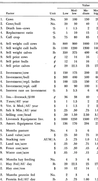
Thirty-nine factors that influence returns to labor and management of a beef cow-calf operation were identified (Table 1). Values for each ranged from low to high based on data from ranchers’ experience, publications in literature cited, and knowledgeable judgment. This range was divided into five equal units, “low,” “medium low,” “medium,” “medium high,” and “high.” Any value may represent a rancher’s three to five year average.
Table 1 is arranged into eight groups as used to figure: (1) herd organization, (2) gross income, (3) livestock investment and interest, (4) miscellaneous livestock expense, (5) pasture charge, (6) hay cost, (7) protein supplement cost, and (8) shelter and building charge.
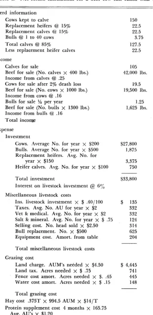
A herd organization model was developed for a 150-cow herd using the “medium” values in Table 1. Forage and feed needs were deter- mined using an adaptation of the summary table (Rasmussen, 1958). The “medium” values of all factors were used to figure income and ex- pense to the nearest dollar for a 150-cow herd (Table 2). The minus return to labor and management is disturbing, but it emphasizes reali- ties. There are, however, plus
312
values such as interest return to land and building investments, and land value appreciation. There may be other long term benefits as ef- fect on water supply, value of land for recreation, and conservation of resources for future generations as pointed out by Ciriacy-Wantrup and Schultz (1957).
The minus return provokes spec- ulation as to changes that could produce a profit. However, the focal point of this project is which factor has greatest influence on net returns. Eight factors were selected for this analysis. They are calf sell- ing weights, calf selling price, per- cent calf crop, hay cost per ton, months grazing versus months hay- ing, stocking rate (forage produc- tion), value of grazed land, and livestock property tax. All except livestock property tax are directly related to resource use. They are considered to have major influence on net income depending on the cost of achieving the changes. Net return was calculated at all five values with “medium” value used for all other factors. Thus the ef- fect of the single factor on net re- turn was projected.
Results
Net returns for a 150.cow herd from different calf sale weights and prices range from a minus $6,141 to a plus of $684 (Table 3). A plus return to labor and management resulted from 450 pound calves at
Table 1. Management factors that influence net income of beef cow-calf
FACTOR COMPARISON 313
ranches and values for each.
Value
Factor Unit Low Med- low dium Me- Med- high High
1.
cows
No. 50 100 150 200 2502. Cows/bull No. 20 30 40 50 60 3. Death loss-cows % 1 1.5 2 2.5 3 4. Replacement ratio % 5 10 15 20 25 5. Calf crop % 75 80 85 90 95 6. Sell weight cull cows lb 800 900 1000 1100 1200
7. Sell weight cull bulls lb 1100 1200 1300 1400 1500 8. Sell weight calves lb 350 375 400 425 450 9. Sell price cows $ 12 14 16 18 20 10. Sell price bulls $ 12 14 16 18 20 11. Sell price calves $ 20 22.5 25 27.5 30 12. Investment/cow $
13. Investment/bull $ 14. Investment/repl. heifer $ 15. Investment/repl. calf $ 16. Interest rate on investment %
200 225 250 500 600 700 150 175 200 100 110 120 6 6.5 7 17. Ins.-livestock/$100 $
18. Taxes/AU year $ 19. Vet. & Med./AU year $ 20. Salt & Min./AU year $ 21. Selling cost/head $ 22. Livestock Equipment Inv. $ 23. Amort. Equipment Cost $
40 42 44 2 2.5 3 2 2.5 3 .75 1.00 1.25 2.50 3.50 4.50 1500 1750 2000 204 238 272 24.
25. 26. 27. 28. 29.
Months pasture No. Land value/acre $
30. 31. 32.
Stocking rate AUM/A Land tax/acre $ Fence cost/acre $ Water cost/acre $ Months hay feeding No. Hay Fed/AU day lb Hay cost/ ton $ Months protein fed No. Protein fed/AU day lb Protein price/ton $ Lvstk. building value $ Amortized building cost $ Building insurance/$100 $ Building maintenance @ 2% $
150 175 300 400 100 125 80 90 5 5.5 36 38 1 1.5 1 1.5 .25 .50 .50 1.50 1000 1250 136 170 4 5 25 50 .5 .75 .25 .50 .15 .30 .05 .lO 4 5 20 22.5 10 12
6 7 8 75 100 125 1.0 1.25 1.5 .75 1.00 1.25 .45 .60 .75 .15 .20 .25 6 7 8 25 27.5 30 14 16 18 33.
34. 35.
2 3 4 5 6 .5 .75 1 .oo 1.25 1.5 70 75 80 85 90 36.
37. 38. 39.
6000 8000 10000 12000 14000 436 581 726 871 1016 45 50 55 60 65 120 160 200 240 280
pounds. This illustrates the inter- for land values and stocking rates, related effect of two variables. percent calf crop and selling price, The same kinds of calculations and for grazing versus haying and were made and tables developed hay price. Net return and differ-
ence also were calculated for differ- ent personal property tax rates on livestock. This is a minor factor for influencing income as evidenced by the magnitude of change needed. When the differences in net in- come were plotted the result was essentially a straight line for sale weight, sale price, cost of hay, per- cent calf crop, and land values. The month’s grazing versus haying line was almost straight. It was gov- erned by small differences in the monthly needs for animal unit months. Differences in net return due to changes in stocking rate pro- duced a curved line. Differences were greater at lower stocking rates than at higher. This is because uni- form stocking rate increment repre- sents a higher percentage change at lower rates.
A common base is essential to compare the impact of different factors. Ten dollars per brood cow was chosen as a meaningful unit for comparison because this differ- ence in income per brood cow in a herd seems significant. The differ- ences resulting if the value of only one factor changed and all others remained at the “medium” value were used in calculating the com- parison. The results are expressed as the amount of change in value of a factor needed to produce a $10 difference in net return per cow. They are 57.2 pounds selling weight per calf; 3.6 cents per pound calf weight sold; 10.3 percent calf crop; $4.02 per ton for hay; 12.2 months of pasture versus hay change with hay at $14.00 per ton, or 4.1 month’s change with hay at $18.00 per ton; 2 AUM’s per acre in stocking rate; $25.30 per acre grazing land value; and $9.04 tax per animal unit.
These figures will not be the same in all situations for the fac- tors shown. The number of month’s change necessary with hay at $14 and $18 per ton illustrates this.
314 BREDEMEIER
Table 2. Net return calculations for a beef cow-calf ranch with 150 cows.
Herd information Cows kept to calve
Replacement heifers @ 15% Replacement calves @ 15% Bulls @ 1 to 40 cows Total calves @ S5%
Less replacement heifer calves
150 22.5 22.5 3.75 127.5
22.5 Income
Calves for sale
Beef for sale (No. calves x 400 lbs.) Income from calves @ .25
Cows for sale after 2% death loss Beef for sale (No. cows x 1000 lbs.) Income from cows @ .16
Bulls for sale % per year
Beef for sale (No. bulls x 1300 lbs.) Income from bulls @ .16
Total income
105 42,000 lbs.
19.5 19,500 lbs.
I .25 1,625 lbs.
$10,500
d 3,120
$ 260 $13,880 Expense
Investment
Cows. Average No. for year x $200 Bulls. Average No. for year x $500 Replacement heifers. Avg. No. for
year X $150
$27,800 1,875
Heifer calves. Avg. No. for year x $100 3,375 750
Total investment $33,800
Interest on livestock investment @ 6y0 $ 2,028
Miscellaneous livestock costs
Ins. livestock investment x $ .40/100 Taxes. Avg. No. AU for year x $2 Vet & medical. Avg. No. for year x $2 Salt & mineral. Avg. No. for year x $ .75 Selling cost. No. head sold x $2.50 Bull replacement. No. x $500 Equipment cost. Amort. from table
$ 135 332 332 124 314 625 204
Total miscellaneous livestock costs $ 2,066 Grazing cost
Land charge. AUM’s needed x $4.50 Land tax. Acres needed x $ .75
Fence cost amort. Acres needed x $. .45 Water cost amort. Acres needed x $ .15
$ 4,445 741 445 14s
Total grazing cost
Hay cost .375T x 994.5 AUM x $14/T Protein supplement cost 4 months x 165.75
Avg. AU’s x $1.20
$ 5,779 $ 5,221
$ 796 Building costs
Building cost Amort. from table Building Ins. value x $ .55/ 100 Building maintenance from table
$ 726 55 200
Total building costs $ 981
Total expense $lS,S71
Net return $-2,991
$4.50 used as a cost per animal unit month for grazing is relatively high when compared to the low cost of
$14 per ton for hay fed at 25 pounds per animal unit day.
This illustrates how low cost hay or other winter feed can help en- hance profits. Such low costs are essential for ranchers in regions with long winter feeding periods. When hay was figured at $12 per ton and grazing at $4.50 per ani- mal unit month, net income to labor and management was not af- fected by changing length of graz- ing and feeding periods.
, This held true under the condi-
tions used in this analysis when cost per ton is 2% times the cost of an animal unit month of grazing. If hay is charged to the livestock enterprise at more than 2.66 times the animal unit month of grazing, the net return to labor and man- agement can be increased by length- ening the grazing season within climatic limitations.
Management changes such as calv- ing dates can influence income as demonstrated by Mueller and Har- ris (1967). Such changes influence income as their effect is reflected in the values of factors. Proper grazing use as contrasted with over- use can increase weights, percent calf crop, and may reduce livestock investment costs based on Soil Con- servation Service experience in working with ranchers. The costs involved in producing the changes in factor values was not included in this analysis. Such costs must be considered in the application of cost and return analysis to resource uses. Individual ranchers must use their values for all factors when ap- plying this procedure to analyzing their problems.
This entire procedure for calcu- lating cost and returns under alter- natives of factors showing return to labor and management for beef cow-calf operations has been pro- grammed on a Soil Conservation Service computer.
FACTOR
COMPARISON
315
Table 3. Net returns and differences (dollars) from different calf sale weights (pound) and selling prices (dollars) based on a 150~cow herd.
Selling
price 350
Calf sale weights Average
dollars/
3’75 400 425 450 25 lbs.
.20 -6141 -5616 -5091 -4566 -404 1 525” .225 -5222 -463 1 -404 1 -3450 -2860 590.5” .25 -4304 -3647 -2991 -2335 -1679 656.5” .275 -3385 -2663 -1941 -1219 - 497 722”
.30 -2466 -1679 - 891 - 104 + 684 787.5”
Average dollars at
.025 per pound 918.75b 984.25b 1050b 1115.5b 1 181.25b * Difference in net income due to 25 pounds change in calf sale weight. b Difference in net income due to 2.5~ per pound change in calf sale price.
in west-central Kansas. Ft. Hays Branch Kan. Agr. Exp. Sta. Bul. 394. LEITHEAD, H. L. 1960. Grass man- agement pays big dividends. J. Range Manage. 13:206-210.
MUELLER, R. G., AND G. A. HARRIS. 1967. Economics of selected alter- native calving dates. J. Range Man- age. 20: 67-69.
OLIVER, J. D., AND R. G. KLINE. 1965. Optimum enterprise combinations for beef cow and calf farms in south- west Virginia. Vir. Agr. Exp. Sta. Tech. Bul. 180.
Ohio Agr. Exp. RASMUSSEN, L. H.
livestock numbers, . .
OLSON, R. 0. 1959. Some opportuni- ties for improving farm income in southeastern Ohio.
Sta. Res. Bul. 832.
on ranching units.
1958. Balancing feed and forage
J. Range Man-
Literature Cited
BEATY, E. R., J. D. POWELL, J. C. FORT- SON, AND F. B. SAUNDERS. 1963. Pro- duction aspects of a beef cow-calf operation on grass pastures. J. Range Manage. 16:250-253.
1965. Fescue pastures, under differ- ent management systems, and or- WHI~ENBERG, AND J. W. HIGH, JR.
chardgrass-clover for yearlong slaugh- ter steer production. Tenn. Agr. Exp. Sta. Bul. 385.
age. 11: 194-197. RIECK, R. E., G. C.
HENQUINET. 1966.
and returns in northern Wisconsin. Wis. Agr. Exp. Sta. Res. Rep. 22. WELLS, A. R., AND S. A. EUGENE. 1966.
Costs and returns of beef cow herds. Minn. Uni. Farm Business Notes No. 489.
CIRIACY-WANTRUP, S. V., AND A. M. SCHULTZ. 1957. Problems involving conservation in range economics re- search. J. Range Manage. 10:12-16. DOANE’S AGRICULTURE REPORT. 1968.
Do you know what it costs to keep a cow? Sep. 8, pp. 20-25.
GERLOW, A. R., AND J. R. CAMPBELL. 1965. Enterprise costs and returns for beef cattle, Southern Louisiana rice area. La. Agr. Exp. Sta. DAE, Res. Rep. No. 337.
HIGH, T. W., JR., E. J. CHAPMAN, B. L.
HOTTELL, J. B., AND A. F. ARNOLD. 1965. Crop pasture, timber and live- stock enterprises for the Boston Mountain and Ozark Highland areas of Arkansas. Ark. Exp. Sta. Rpt. Series 135, pp. 13-66.
KEARL, W. A. 1961. Cattle ranching in the Northern Plains area of Wyo- ming. Wyo. Agr. Exp. Sta. Mimeo Cir. No. 155.
LAUNCHBAUCH, J. L. 1957. The ef- fect of stocking rate on cattle gains and on native shortgrass vegetation
PULVER, AND W. Beef cow costs
WESTERN, C., AND A. W. EPP. 1965. The Nebraska sandhills ranch busi- ness, 1965 summary. Nebr. Uni., Agr. Col. Agr. Econ. Dep. Memo. WILLHITE, F. M., AND A. R. GRABLE.
1966. Greater profit from livestock in the intermountain west with effi- cient ranch management. J. Range Manage. 19: 112-l 18.
THESIS: UNIVERSITY OF WYOMING
Diet Preference and Utilization Patterns of Elk in the Northern Big Horn Mountains, Wyoming,
by George
E. Probasco. M.S. Range Management, 1968.Data were collected during the summer of 1967, on die- tion between elk grazing patterns and percent total basal tary preferences and grazing patterns of elk in the northern
Big Horn Mountains of Wyoming. Forest openings, where cover of herbaceous vegetation.
only elk grazing occurred, were studied to determine pre- Data on diet preferences indicated that elk utilized grasses ferred plant species for both the spring and summer seasons. during the spring period but shifted their preference to
One forest opening of approximately 300 acres was strati- forbs during the summer season. Preferred species for the fied to determine if there was a correlation between elk spring period were Bromus margin&us, Bromus spp., Fes- grazing patterns and distance from forest margin. Elk graz- tuca idahoensis~ and I’Oa sPP* Preferred species for the
Land Management Policy
and Development of Ecological Concepts
1DONALD A. JAMESON
Associate Professor of Range Science, College of Forestry and Natural Resources,
Colorado State University, Fort Collins.
Highlight
As ecological concepts become incor- porated into the training and back- ground informat,ion of professional land managers, they also become in- corporated into land management policies. Recent developments in ecol- ogy, such as nutrient cycling studies and computer simulation of complex processes, have a favorable climate for acceptance. Possible applicatcions should be carefully studied by land managers.
It is certainly paradoxical that in a world filled with hunger, the United States is constantly faced with the need to hold back on agri- cultural production. It is also dis- turbing to many of us who have worked for years to increase live- stock production on rangelands that our efforts in this direction, al- though desirable from an individ- ual viewpoint, are no longer critical from the national viewpoint. It is particularly frustrating because we have the technology to double or perhaps triple the production from our rangelands. Because of these facts, range managers have, in many cases, lost their sense of mission.
There are, however, more and perhaps greater things which need doing. I like to classify the jobs
lWork presented in this paper was supported in part by National Science Foundation Grant GB-7824 for the Analysis of Structure and Function of Grassland Ecosystems. Many of the ideas expressed in this paper are the result of discussions with several of the investigators in the Grassland Biome subprogram of the Interna- tional Biological Program, particu- larly L. J. Bledsoe and G. M. Van Dyne. Received January 23, 1970; ac- cepted for publication May 8, 1970. 2The author is Director of the Pawnee
Site project in the Grassland Biome program of the U.S. International Biological Program.
facing range managers today into the categories of (1) scientific un- derstanding of the resource, (2) technological efficiencies (as op- posed to technological possibilities), and (3) rural social adjustments. This order is not intended to assign any priorities to these three tasks; all are deserving of full considera- tion. This paper, however, will deal only with scientific understanding of the resource.
Theories are basic tools of science; all scientists need theories on which and with which to operate. It mat- ters little whether the theory is cor- rect, it must, however, be useful. Consider, for example, earlier theo- ries of electron flow. Much elec- tronic equipment was first designed with the belief that electrons flow in a certain direction around a cir- cuit. As it turns out, electrons actu- ally flow in exactly the opposite di- rection; nevertheless, circuits based on the original theory do work. Many other examples of operable, but inaccurate, theories exist. A theory, therefore, is to be judged not on the basis of truth, but on the basis of its usefulness. As long as the theory is useful, it very likely will not be replaced, but when the theory is no longer useful, it will eventually be replaced. The em- phasis in this paper, for example, is intended to be provocation rather than accuracy, and hopefully the paper will have a short life.
Ecological Concepts of Existing Policies
Some early theories of ecology were developed from observations on the peat bogs of Europe, where
several observers felt that the bogs developed through well defined stages. This reasoning was perhaps
most notably followed in the United States by Clements (1916), who with Weaver (Weaver and Clements,
1938) developed a strong school of successional ecology based largely on observations in the sandhills of Nebraska. Clementsian ecology became the focal point of U. S. ecol- ogy for many years, and certainly received much impetus from the very practical management needs that were pointed out during the “dust bowl” days of the 1930’s. Clementsian ecology, and other viewpoints of successional ecology, propounds that we first begin with bare rock which is converted by stages. These stages may include lichens and mosses, annual plants, perennial forbs, grasses, and finally, in appropriate climates, shrubs or trees. Such a progression is known as a xerosere. On the other hand, hydroseres, beginning with water but ending with the same climax condition, also can occur. If the progression from rock or water to the climax community is set back by any disturbance, and progres- sion is then allowed to resume, the resumption of succession is known as secondary succession.
Most land managers in the United States today who are in a position to make policy decisions were most likely trained in successional ecol- ogy. In fact, concepts of succes- sional ecology have been written into policy statements of many land management and advisory agencies. In some agencies, Clementsian ecol- ogy has become so entrenched in service policy that any one speak- ing out against these concepts, or even offering additional concepts, is considered a heretic.
Theories of successional ecology certainly have been useful. It was, for example, a most useful and necessary tool to recover from some of the earlier abuses in range man- agement in the western United States. Certainly in many areas we have a long way to go before we can completely exhaust the benefits from successional ecology and its concepts. We have, however, con- tinued to use successional ecology
POLICY AND ECOLOGY 317
over and over until it has lost much of its usefulness. Much of the west- ern range is in a condition where great progress from secondary suc- cession alone cannot be expected. Most ranges are in much better condition than they were earlier, and we certainly have the necessary basic technology, if not the eco- nomic efficiency and political abil- ity, to finish this particular job. In addition, Clementsian “sand hill” ecology has been pressed into use in areas where it was not conceived and where it is not quite so ap- propriate. Perhaps a few examples would be in order. In timbered lands, for instance, the progression towards climax does not necessarily equal a progression towards better conditions for range livestock. In fact, a climax coniferous forest is usually in very poor “range condi- tion.” On the other hand, a well established and well managed seeded range, by definition, is in a disclimax state because all of the species present are invaders, but, from the productivity standpoint, it may be excellent.
Although theories of successional ecology are still used by land man- agement agencies, many range re- searchers have long since aban- doned this concept as a fruitful area of research. They have, in- stead, turned to such fields as plant physiology, animal nutrition, and agronomy (including reseeding and brush control). This shift to simi- lar, but more restricted, fields has, in part, been promoted by educa- tional institutions which have been unable to offer solid training in range science as a total system con- cept. This search for meaningful research fields has led, in many cases, to fragmented research pro- grams without a central theme, and has occasionally produced dichoto- mies between researchers and land managers.
Recent Trends in Ecology
Useful as successional ecology has been, it has become somewhat shop worn and is now being replaced on the theoretical front by a wide ar-
ray of concepts and mathematical techniques and approaches collec- tively known as systems ecology. Since the term is used to describe a potpourri of the interesting and uninteresting, valid and invalid, and meaningful and meaningless, it would be impossible to cover sys- tems ecology in a brief presenta- tion. It is, however, possible to out- line what seems a dominant concept as indicated by current interest of the scientific community, the prob- ability of significant contributions of basic knowledge, and the validity of the use of the term systems ecology.
Tansley ( 1935) introduced the term “ecosystem” into the English language literature. Tansley’s in- troduction of the term, however, was mostly a definition and it re- mained for Lindeman (1942) to clearly outline trophic (i.e., feeding level) ecology which has, in recent years, become a central theme for much ecological research. Linde- man happened to be an aquatic ecologist, and his paper on the trophic-dynamic aspects of ecology uses examples from aquatic com- munities. Nevertheless, the prin- ciples he outlined apply generally to other ecological systems.
Lindeman said that an ecosystem is a system made up of various com- partments; the compartments are called trophic (feeding) levels and ordinarily include producers (or, more commonly, green plants), con- sumers (which in turn can be sub- divided into primary consumers which eat plants, secondary con- sumers which eat primary consum- ers, etc.), and decomposers (which convert dead plant and animal matter back into carbon dioxide). Energy is received from the sun, and energy and matter are trans- ferred among the various compart- ments. If we truly understood this transfer of energy and matter, we would then truly understand the operation of the system. If we un- derstood these transfers so well that we could express them mathemati- cally, we could then examine the effects of many manipulations of
the ecosystem and predict many results without actually doing field experiments.
If we think about the few simple compartments outlined above (pro- ducers, consumers, and decompos- ers), we see that we could readily subdivide these compartments into growth forms, species, individuals, or parts of individuals. We could also consider many kinds of matter. Thus our concept of the ecosystem could very readily become entirely too complex to handle by ordinary bookkeeping systems. In addition, the measurements of transfers from one compartment to the other are in many cases quite difficult, and in Lindeman’s time may have been impossible. In fact, many of them are still impossible, but introduc- tion of radioisotopes as tracers and many sophisticated instruments have greatly facilitated and pro- moted studies of transfer processes. For these very pragmatic reasons, therefore, trophic-dynamic ecology did not immediately arise to the forefront after Lindeman’s original exposition. In fact, most of those attending universities over 20 years ago probably did not hear of trophic-dynamic ecology.
318
iar with computer techniques. The development of mathematical tools used in analysis of feedback control systems is especially useful, and it it from this field particularly that much of the terminology of systems ecology is being drawn. An “adap- tive control system with stochastic inputs” (Rosen, 1967), for example, sounds exactly like an ecological situation. The concept of an adap- tive system, in fact, provides for union of the theories of successional ecology with the theories of trophic ecology if we consider an ecological system which is undergoing succes- sion as a self-organized system (Margalef, 1968).
We now find arising today a con- siderable number of mathemati- cally-oriented biologists, and bio- logically-oriented mathematicians and engineers, who are attacking the problem of trophic-dynamic ecology. It is something of a basic ground swell among ecologists. In fact, we can say with certainty that complex ecological systems will be investigated from the standpoint of trophic-dynamic ecology and sys- tems engineering. The only ques- tion, since science does progress as a body, is who is going to do it best.
It happens that at the moment the primary worldwide research ef- fort in this area is centered about the International Biological Pro- gram (IBP). Particularly in the U. S. these efforts are imbedded in the integrated IBP research pro- gram on the Analysis of Ecosystems (AOE). A number of IBP Biome programs have been organized within the AOE including the Grassland, Desert, Eastern Decidu- ous Forest, Western Coniferous Forest, Tundra, and Tropical Biomes. Of these biome programs, the Grassland was selected for the first major effort because of (i) its seeming simplicity, (ii) the location of a suitable intensive study area, namely the combined areas of the Pawnee National Grassland and the Central Plains Experimental Range, known in IBP circles as the Pawnee Site, (iii) the rapid and ex- tensive cooperation of a suitable
JAMESON
from (time t )
FIG. 1. A matrix of transfers between compartments of closed system. Here, 0 = no transfers, -1 = diagonal elements, and + = transfer between compartments. The sum of all positive numbers in the columns of this figure will be +l, so that for closed systems at steady state the total transfer to each compartment will sum to zero.
Cl Live plonts
C, Standing dead
C, Plant litter
C, M icrof lora
C, Soil Organic Matter
C, Herbivores
C, Omnivores
C, Carnivores
C, Soil fauna
C,, Animal litter
pool of scientific manpower avail- able at the several major nearby universities and colleges and associ- ated federal research organizations, and (iv) the obvious dependence of man on the grasslands of the world.
Matrix Representation of Ecosystems
We have stated above that an eco-
system is a system which transfers energy and matter from one com- partment to another (for a further discussion see Margalef, 1968). If we have “n” such compartments, we can describe a greatly simplified ecosystem as a “n x n,” who-eats- whom matrix in which the ele- ments of the matrix describe the rate of transfer of energy or matter
from each compartment at time “t” to each of the compartments at time “t + At” (Fig. 1). If we knew
the individual coefficients or math- ematical functions for all such transfers in this matrix, we could then claim to understand the func- tion of the ecosystem. In Fig. 1, I have entered some zero coefficients, but scientists involved in the study
of various transfers will make the case that, in the strictest sense, there are very few zero transfers. At this point, however, the matrix is most important to point out an ap- proach.
Ingestion of herbage by herbi- vores is one transfer process-in this case the transfer between live plants and a particular herbivore species. The rate of this transfer process becomes an element in our who-eats-whom matrix. Biologists have been working on the deter- mination of many of these transfers for some time, but others have not received a great deal of attention. In fact most of the energy and mat- ter transfers cannot be measured directly. Therefore if we are to say that we understand an ecosystem by knowing where energy and matter flows in the system, we must find some other procedure.
An Analytical Approach