Sliding Mode Control with Observer and Application

(1)

ISSN (Print) : 2320 – 3765 ISSN (Online): 2278 – 8875

I

nternational

J

ournal of

A

dvanced

R

esearch in

E

lectrical,

E

lectronics and

I

nstrumentation

E

ngineering

(An ISO 3297: 2007 Certified Organization)

Vol. 5, Issue 10, October 2016

Sliding Mode Control with Observer and

Application

B.Shanmugam, Dr.K.Balagrurunathan

Professor, Dept. of EEE, St. Peter’s University, Avadi, Chennai, India

Advisor, St. Peter’s University, Avadi, Chennai, India

ABSTRACT: This paper focuses essentially on the classical variable structure control (VSC), also known as sliding mode control (SMC) theory in sec.2. Initially, the paper introduces the classical principle of sliding mode control method. Standard sliding modes provide for finite-time convergence, precise keeping of the constraint and robustness with respect to internal and external disturbances is highlighted by example 2.1 .

The structure of the control law changes due to the location of the state trajectory in the state space according some switching function. The switching function is designed in order to attract the trajectory in the state space to the switching surface.

However, often they also exhibit a serious drawback which essentially hinders their practical applications. This drawback – high frequency oscillations which inevitably appear in any real system is usually called chattering in fig 2.2. This is a highly undesirable phenomenon, because it causes serious wear and tear on the actuator components. To avoid chattering and estimation of un-measurable states of the systems, Sliding Mode observer is proposed and explained using example

KEYWORDS: Variable Structure Control, Sliding Mode Control, signum function,

I. INTRODUCTION

Variable Structure Control (VSC) or Sliding Mode Control (SMC) was proposed in the early 1950s (Utkin, 1965), (Emelyanov, 1967), (Itkis, 1976), (Utkin, 1977),(Utkin, 1978). Over the past several decades, increasing attention has been drawn to VSC or SMC and hitherto, significant approaches have been developed world widely (Young, 1977).SMC is one of the well-known robust control design methods which only require the upper bounds of the parametric uncertainties and Thus the prescribed specifications would be met through these two designing stages in SMC.

In SMC, switching control using signum function is one of the best control strategies to handle the worst case control disturbances. Due to the simplicity and superb robustness of SMC, numerous successful applications have been carried out to a wide variety of engineering systems, such as electric drives, robotic manipulators, etc. (Slotine and Sastry, 1983). In terms of Filippov’s work (Filippov, 1964), (Filippov, 1988), in which the author derived a formal justification which is one possible technique for determining the system motion in a sliding mode, the properties and the definition of the sliding mode have been well presented in detail in (Utkin, 1978) and (Utkin, 1992). A standard SMC controller is designed in two stages. One is the sliding manifold or switching surface. The essential feature of the sliding mode control is the choice of a switching surface of the state space according to the desired dynamical specifications of the closed-loop system. The plant dynamics restricted to this surface or manifold represent the controlled system’s behavior. The other is the discontinuous control law which is designed to steer the trajectories onto the sliding manifold in finite time and to keep the subsequent motion on it. In the ideal case, the resulting motion is called sliding mode. The main advantages of the sliding mode control are:

1) The resulting systems have their insensitivities or robustness against a large class of perturbations or model uncertainties, which enter the system in the same channel as control inputs.

(2)

I

nternational

J

ournal of

A

dvanced

R

esearch in

E

lectrical,

E

lectronics and

I

nstrumentation

E

ngineering

implementation. The actuators have to cope with the high frequency bang-bang type of control actions that could produce premature wear, or even breaking. This main disadvantage, called chattering, is generally perceived as an oscillation about the sliding manifold which may excite the unmolded high frequency dynamics of the plant and is harmful to actuation mechanism. The chattering can be reduced or even suppressed by using techniques such as nonlinear gains, dynamics extensions and higher order sliding mode control (Zinober, 1994), (Bartolini,1996), (Fridman and Levant, 1996).

II. SLIDING-MODE CONTROL THEORY

This work deals with a special class of systems, called “variable structure systems” (VSSs), that are of great importance in systems and control theory. As described by Utkin (1977) the basic concept of VSCs is that the system is allowed to change structure at any instant. The design problem in VSCs is therefore to find the parameters in each of the system structures and to design the switching logic which decides when the structure of the system should change. One of the key features of Variable Structure Systems is that the resulting system can show properties not present in any of the separate system structures. The motion described by these trajectories is known as sliding mode.

The response of a system with sliding mode control can basically be divided into two parts

1. The reaching phase: When s ≠ 0, the system is said to be in the reaching phase. The trajectories in the phase plane will in this phase move toward S.

2. The sliding phase: Once the system reaches S the trajectories will move along the surface described by S until it reaches the equilibrium point.

A. ANALYTICAL APPROACH TO SLIDING-MODE CONTROL

It is now necessary to formulate the general mathematical description of Sliding-Mode Control with the preconditions of its occurrence and retention. A plant to be controlled can be described in general as the following matrix differential equation:

̇ (t) = A (t, x) + B (t, x) u (t) (2.1) where x is state vector, t is continuum (time), A is system matrix, B is system input matrix and u is control vector of

length m. According to the Sliding-Mode Control methodology the control vector u must be determined:

= ( , ) ( ) > 0

( , ) ( ) < 0 i = 1,2 …m (2.2)

where s(x) is a vector containing m switching functions.

The switching functions are defined to meet the following requirements;

1. during reaching-mode the state trajectory reaches the sliding surface determined by the matrix equation s (x) = 0. 2. the sliding surface s (x) = 0 is to be carefully designed so that the closed-loop system dynamics tracks its desired transient.

3. the control vector u (x, t) is appropriately selected so that the state vector x, that is in initial instant located outside the switching surface s (x) = 0, is attracted to this surface and reaches it in finite time. Then the rapid switching between the control structures is initialized and introduces the system into sliding-mode.

Hence the state vector x slides on the switching surface s (x) = 0 towards the origin until the perturbed system reaches the equilibrium. Thus it is unequivocal that during sliding-mode the closed-loop system is globally asymptotically stable. The sliding motion equation is of reduced order and depends on neither the plant parameters nor the external disturbances.

B. EXISTENCE AND UNIQUENESS OF SOLUTION

(3)

I

nternational

J

ournal of

A

dvanced

R

esearch in

E

lectrical,

E

lectronics and

I

nstrumentation

E

ngineering

In order to overcome this constraint special functions called vector functions have been proposed by Filippov (Filippov, 1988). A system to be controlled is described by the following differential equation:

̇ = f (x, u) (2.3) The proposed Sliding-Mode Control system with variable structures triggered along the switching surface s(x) = 0 can

be described as follows:

f (t, x) = ( , ), ( ) > 0

( , ), ( ) < 0 (2.4)

According to the equation (2.3) it can be noticed that the system dynamics exactly on the switching surface s (x) = 0 is not defined. Following the Filippov’s idea the behavior of the system can be described as the average value of the both structures (vector fields) in the equation (2.4):

̇(t) = (t, x, u) = + (1 – ) ,

0 ≤ ≤ 1 (2.5) where = f(t, x, u+), = f(t, x, ) and is the resulting velocity vector of the state trajectory while in sliding mode. The term is a function of the system state and can be specified in such a way that the "average” dynamic of is tangent to the surface s(x) = 0. The geometric concept is illustrated in Fig. 2.1.

Fig.2.1. Filippov’s idea of analytical pproach to Sliding-Mode Control As it was initially assumed the system is not defined for the s (x) = 0 but the vector fields and are well-defined in case when the system approaches the sliding surface bilaterally, which can be presented:

= → ( , , ) (2.6)

= → ( , , ) (2.7)

Since it is necessary that the system trajectories in the vicinity of the sliding surface s(x) =0 are oriented towards it, the sufficient condition for the sliding-mode existence can be derived from the equations (2.4), (2.6) and (2.7):

→ ( ) < 0 (2.8)

→ ( ) > 0 (2.9)

The conditions (2.8) and (2.9) ensure that the terminal point of the system state vector that draws the system trajectory does not leave the sliding surface. In sliding-mode it is being affected by the averaged vector field f0 (t, x, u). Moreover the averaged vector field f0 (t, x, u) in each point of the sliding surface

s(x) = 0 must be tangent to this surface in order to preserve sliding-mode.

C. EQUIVALENT CONTROL METHOD

Developed by V.Utkin [Utkin ‘92], the analytical nature of such method makes it a powerful tool for both analysis and design purposes, is detailed with the implications of such methodology, that allows one to go deep inside the core of the VSS theory. It can be shown that the equivalent control method produces the same solution of the Filippov continuation method if the controlled system is affine in the control input, while the two solutions may differ in more general nonlinear cases. Consider system (2.1) with discontinuous control (2.2), and assume that a sliding mode on the manifold s (x) = 0 occurs. Essentially, the equivalent control method establishes that the solution of system (2.1), (2.2) on the manifold s (x) = 0, can be defined as

̇ = f (x, t, ueq) (2.10) where ueq(x, t) is a continuous control action, called “EQUIVALENT CONTROL”, which is the solution of the equation.

(4)

I

nternational

J

ournal of

A

dvanced

R

esearch in

E

lectrical,

E

lectronics and

I

nstrumentation

E

ngineering

is necessary to differentiate the predefined sliding surface s(x) = 0, which means that the system trajectory remains on this surface, if:

̇( ) = = ̇ =

( ) + ( ) = 0 (2.11)

Solving the equation (2.11) over u(x) the equivalent control can be derived in a form of the following matrix equation:

( , ) = ( ) ( ) (2.12)

The solvability of the equation (2.11) is conditioned by the invertibility of the system input matrix B(x). Taking into account the equation (2.2) that defines a variable structure control the system remains in sliding-mode when the equivalent control signal satisfies the following condition:

( , )< ( , )< ( , ) (2.13)

D. PROBLEMS OF REACHABILITY AND STABILITY IN SLIDING-MODE CONTROL

It is recommended first to establish sufficient conditions that will guarantee the occurrence of ideal sliding-mode before designing of the detailed variable structure control for a specific application. The principal conditions (2.8) and (2.9) for sliding-mode existence assumes that the system state trajectories in a certain domain enclosing the switching surface s must be directed towards this surface. This can be also described by the following equivalent criterion

̇ < 0 (2.14) The equations (2.8), (2.9) and (2.14) are called reachability conditions. If the reachability condition (2.14) is valid

globally it leads to the equation: ̇ (t) = ̇

(2.15) where ̇ (t) is a time-derivative of the Lyapunov-like function for the states:

̇ (t) = (2.16) Due to the fact that the reachability condition described by (2.14) guarantees only reaching of the sliding surface in

asymptotic manner the stronger condition called the -reachability condition has been introduced

̇ ≤ − | | (2.17) where is a positive constant. Substituting the Lyapunov-like function gives:

≤ − | | (2.18) Then the time-integral from (2.17) within 0 to ts results as follows:

| ( )|− | (0)| ≤ − (2.19)

Hence the time ts necessary to reach s(x) = 0 satisfies the inequality:

≤ | (0)|

The inequality (2.19) can be considerably concluded that for each time instant t that is greater than ts the system in

sliding-mode is asymptotically stable and insensitive to outer disturbances or system parameter mismatch.

III. CHATTERING PHENOMENON

As already mentioned, the major advantage of Sliding-Mode Control is the insensitiveness to plant parameter variations and disturbances, during sliding mode, which in fact eliminates the necessity of accurate modeling. This nonlinear control technique is an efficient tool of designing of the robust controllers for the complex high-order nonlinear plants operating under the model uncertainties.

(5)

I

nternational

J

ournal of

A

dvanced

R

esearch in

E

lectrical,

E

lectronics and

I

nstrumentation

E

ngineering

Fig.2.2. Real Sliding-Mode Control with chattering of the plant described by (2.20) Fig.2.2. Reaching-mode and ideal sliding-mode of the controlled plant described by (2.20)

EXAMPLE 2.1: Let us consider an example to explain the above steps arrived by means of an example. The set of the following equations has been chosen to describe the second-order nonlinear plant:

̇ =

̇ = ( , ) +

(or) ̇ = ( , , ) + (2.20) with initial conditions, x (0) = x and x (0) = x . where |b| < 1, k > 0 are the constant parameters of the plant, x1,

x2 are state variables (error and its derivative) and u is the control signal and the disturbance term f (x1, x2, t)

= ( , ) , which may comprise dry and viscous friction as well as any other unknown resistance forces, is assumed to be bounded, i.e., | ( , , )| ≤ L > 0.

The problem is to design a feedback control law u = u (x1, x2) that drives the mass to the origin asymptotically. In other

words, the control u = u (x1, x2) is supposed to drive the state variables to zero: i.e., lim→∞ , = 0 and the definition of the sliding surface which is the track to be mapped by the system trajectory while converging towards the origin. In case of the considered second-order plant the switching surface is reduced to the switching line and defined by the differential equation (2.21):

s = c + ̇ (2.21) where c is the positive constant slope of the switching line s = 0. Then the control signal u is assumed as shown in the

equation (2.22):

Since ( ) = ̇ ( ), a general solution of Eq. (2.21) and its derivative is given by

( ) = (0) exp(− )

( ) = ̇ =− (0)exp(− ) (2.22)

both ( ) and ( ) converge to zero asymptotically. Note, no effect of the disturbance f (x1, x2, t) on the state

compensated dynamics is observed. How these compensated dynamics could be achieved? First, we introduce a new variable in the state space of the system in Eq. (2.20):

= ( , ) = + , c > 0 (2.23)

In order to achieve asymptotic convergence of the state variables x1, x2 to zero, i.e.,lim→∞ , = 0 with a given convergence rate as in Eq. (2.22), in the presence of the bounded disturbance f (x1, x2, t), we have to drive the variable s

in Eq. (2.23) to zero in finite time by means of the control u. This task can be achieved by applying Lyapunov function techniques to the s -dynamics that are derived using Eqs. (2.20) and (2.23):

ṡ = cx + f(x , x , t) + u, s(0) = s (2.24)

For the s - dynamics (2.24) a candidate Lyapunov function is introduced taking the form

V = (2.25) In order to provide the asymptotic stability of Eq. (2.24) about the equilibrium point = 0, the following conditions

(6)

I

nternational

J

ournal of

A

dvanced

R

esearch in

E

lectrical,

E

lectronics and

I

nstrumentation

E

ngineering

(a) ̇ <0 for ≠0

(b) lim| |→∞ = ∞

Condition (b) is obviously satisfied by V in Eq. (2.25). In order to achieve finite-time convergence (global finite-time stability), condition (a) can be modified to be

̇ ₌ _{̇ ≤ −} _, _{> 0} _(2.26)

Indeed, separating variables and integrating inequality (2.26) over the time interval 0 ≤ ≤ , we obtain

( )≤ − + (0) (2.27) Consequently, V (t) reaches zero in a finite time tr that is bounded by

≤ ( ) (2.28) Therefore, a control u that is computed to satisfy Eq. (2.26) will drive the variable s to zero in finite time and will keep it at zero thereafter. The derivative of V is computed

V̇ = sṡ= s(cx + f (x , x , t) + u (2.29)

Assuming u =− + v and substituting it into Eq. (2.29) we obtain ̇ = s ( ( , , ) + ) =

s ( , , ) + ≤ | | + (2.30)

Selecting v =− sign (s) where

sign (s) = 1

−1

> 0

< 0 (2.31)

and sign (0) ∈[−1, 1] (2.32) with > 0 and substituting it into Eq. (2.30) we obtain

̇ ≤ | | + | | =−| |( − ) (2.33) Taking into account Eq. ((2.25)), condition ((2.26) can be rewritten as

[ ̇ ≤ − = ̇= −

√ | | > 0(2.34) Combining Esq. (2.33) and (2.34) we obtain

̇ ≤ −| |( − ) =−

√ | | (2.35)

Finally, the control gain is computed as = +

√ (2.36)

Consequently a control law u that drives to zero in finite time (2.28) is

u = − − ( ) (2.37)

Remark 2.1. It is obvious that ̇ must be a function of control u in order to successfully design the controller in Eq. (2.26) or (2.37). This observation must be taken into account while designing the variable given in Eq. (2.23).

Remark 2.2. The first component of the control gain Eq. (2.36) is designed to compensate for the bounded disturbance f (x1, x2, t) while the second term _√ is responsible for determining the sliding surface reaching time given by Eq.

(2.28). The larger the , the shorter, the reaching time. Now it is time to make definitions that interpret the variable (2.23), the desired compensated dynamics (2.20), and the control function (2.37) in a new paradigm.

Definition 1.1. The variable (2.23) is called a sliding variable

Definition 1.2. Equations (2.20) and (2.23) rewritten in a form = + = 0. c > 0

corresponds to a straight line in the state space of the system (2.20) and are referred to as a sliding surface. Condition (2.26) is equivalent to s ̇ ≤ −

√ | | is often termed the reachability condition. Meeting the reachability or existence condition (2.26) means that the trajectory of the system in Eq. (2.20) is driven towards the sliding surface (2.21) and remains on it thereafter.

Definition 1.3. The control u = u (x1, x2) in Eq. (2.37) that drives the state variables x1, x2 to the sliding surface (2.23)

in finite time , and keeps them on the surface thereafter in the presence of the bounded disturbance f (x1, x2, t), is

(7)

I

nternational

J

ournal of

A

dvanced

R

esearch in

E

lectrical,

E

lectronics and

I

nstrumentation

E

ngineering

IV. SLIDING MODE OBSERVER/DIFFERENTIATOR

So far, we have assumed that both state variables ( ) and ( ) are measured (available). In many cases only (a position) is measured, but (a velocity) must be estimated. In order to estimate (assuming a bound on | | is known) the following observation algorithm is proposed:

̇ = (4.1)

where v is an observer injection term that is to be designed so that the estimates → and → . Let us introduce an estimation error (an auxiliary sliding variable)

= − (4.2)

Subtracting the first equation in Eq. (2.20) from Eq. (4.1) we obtain

̇ = − + (4.3) Let us design the injection term v that drives = − →0 in finite time. In this case

will converge to x1 in finite time. The following choice of injection term

= − ( ), > | | + , > 0 (4.4) yields

̇ = (− − ( ) ≤ | |(| |− )

≤ − | | (4.5)

Inequality (4.5) mimics Eq. (2.34)/ (2.17), which means that in a finite time tr ≤ | ( )|

→0 or ̇ → . Therefore, a sliding mode exists in the observer (4.1) for t ≥ tr. The sliding mode dynamics in Eq. (4.3) are computed using the concept of equivalent control studied in Sect.2.3.

̇ = − + = (4.6)

What about estimating ? It is clear from (4.6) that the state variable can be exactly estimated as = , ≥ (4.7) The equivalent injection can be estimated by LPF of the high-frequency switching control (4.4) as ̇ = − − ( ) (4.8) where is a small positive constant, and finally

≅ − , ≥ (4.9)

Remark 1.3. The sliding mode observer given by Eqs. (4.1), (4.4), (4.8), and (4.9) also could be treated as a differentiator, since the variable it estimates is a derivative of the measured variable

(8)

I

nternational

J

ournal of

A

dvanced

R

esearch in

E

lectrical,

E

lectronics and

I

nstrumentation

E

ngineering

Fig.4.4. Sliding variable

Example 1.6. The system (2.20) with the sliding mode control (2.37), the initial conditions (0) = 1, (0) = 2 , the control gain = 2 , the parameter = 1.5 , and the disturbance ( , , ) = sin(2 ), which is used for simulation purposes only, is simulated. The variable is measured, and the variable is estimated using the sliding mode observer (4.1), (4.4), (4.8), and (4.9) with =10 and = 0.01 . The results of the simulations are shown in Figs.4.1.– 4.4

Fig.4.1. Estimating x2

(9)

I

nternational

J

ournal of

A

dvanced

R

esearch in

E

lectrical,

E

lectronics and

I

nstrumentation

E

ngineering

The sliding mode observer given by Eqs. (4.1), (4.4), (4.8), and (4.9) estimates x2 very quickly and very accurately

(Figs. 4.1 and 4.3). The sliding variable (1.5) with x2 replaced by its estimate , = + 1.5 , converges to zero in

finite time tr ≈ 1 s. Furthermore the state variables , →0 as time increases (see Fig.4.2) despite the presence of the bounded disturbance

f ( , , t) = sin (2t).

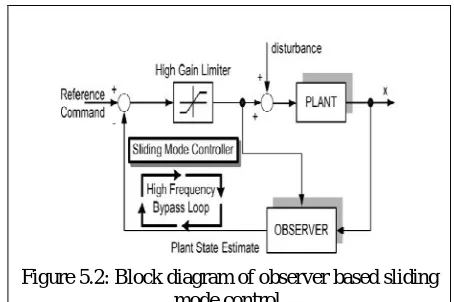
Figure 5.2: Block diagram of observer based sliding mode control.

V. CONCLUSIONS

The classical theory of Sliding Mode Control is analyzed. The presence of modeling imprecision f ( 1, 2 t), can be overcome by the sliding mode controller, using linear sliding function (x). To overcome the problem of unavailable state variables for control the proposed Observer-based sliding mode estimator, we are able to design sliding mode estimator that rejects disturbance. Both systems are found to perform robust way rejecting modeling imperfections and external disturbances and estimating unavailable states in a remarkable way.

REFERENCES

1. A. Levant. Sliding mode control. International Journal of Control, 58(6):1247–1263, 1993.

2. Slotine J. J. E., “Sliding controller design for nonlinear systems”, International Journal of Control, Vol. 40, pp. 421-434, 1984.

3. A. J. Fossard T. Floquet. Sliding Mode Control in Engineering, chapter Introduction: An Overview of Classical Sliding Mode Control, pages 1–27. Marcel Dekker, Inc., 2002

4.S.V.Emelyanov,.BinaryAutomatic Control Systems, Translated from the Russian, Mir Pub. 1987

5. V.I.Utkin, Sliding modes and their application in variable structure systems, Translated from the Russian Mir Pub. 1978,

4.Bartolini, D.; Ferrara, A. & Usai, E. (1998). Chattering avoidance by second-order sliding mode control. IEEE Trans. on Automatic Contr. Vol., 43, 241–246

5.DeCarlo, R S.; Żak S. & Mathews G. (1988). Variable structure control of nonlinear multivariable systems: a tutorial. Proceedings of the IEEE. Vol., 76, 212–232

6.Edwards C. & Spurgeon, S. K. (1998). Sliding mode control: theory and applications. Taylor and Francis Eds

7.Hung, J. Y.; Gao W. & Hung, J. C. (1993). Variable structure control: a survey. IEEE Trans. On Ind. Electron. Vol., 40, 2–22 8.Levant, A. (1993).Sliding order and sliding accuracy in sliding mode control. Int. J. of Contr.Vol., 58, 1247–1263