3D eclipse mapping in AM Herculis systems - ‘genetically modified fireflies’

3D eclipse mapping in AM Herculis systems – ‘genetically

modified fireflies’

Pasi Hakala,

Mark Cropper

and Gavin Ramsay

2_{Mullard Space Science Laboratory, University College London, Holmbury St Mary, Dorking, Surrey RH5 6NT}

Accepted 2002 April 18. Received 2002 April 17; in original form 2002 February 12

A B S T R A C T

In order to map the three-dimensional location and shape of the emission originating within the accretion stream in AM Her systems, we have investigated the possibilities of relaxing the hitherto-applied constraint of a predetermined stream trajectory in modelling the eclipse pro-files. We use emission points which can be located anywhere in the Roche lobe of the primary, together with a regularization term which favours any curved stream structure, connected at the secondary and white dwarf primary. Our results show that, given suitable regularization constraints, such inversion is feasible. We investigate the effect of removing the regularization term, and also the sensitivity of the fit to input parameters such as inclination.

Key words: accretion, accretion discs – methods: data analysis – binaries: eclipsing – novae, cataclysmic variables.

1 I N T R O D U C T I O N

AM Herculis systems (or polars) are a subclass of cataclysmic vari-ables (CVs) in which a magnetic white dwarf accretes matter from a late-type dwarf secondary via Roche lobe overflow. The strong (10–100-MG) magnetic field of the white dwarf prevents the for-mation of an accretion disc, and thus accretion proceeds through an accretion stream that directly impacts on to the white dwarf sur-face near the magnetic poles (see Cropper 1990 for a review on polars).

Until the early 1990s it was widely accepted that almost all the optical emission from AM Her systems originates in the cyclotron emission region(s) near the magnetic poles of the white dwarf. How-ever, the discovery of highly-asymmetric optical eclipse profiles in systems like HU Aqr (Hakala et al. 1993; Schwope, Thomas & Beuermann 1993) demonstrated that the accretion stream could con-tribute as much as 50 per cent of the total optical emission. Since then a number of attempts have been made to use the eclipse profile infor-mation of the AM Her systems to reconstruct the location and other properties of the stream emission. These earlier attempts include those of Hakala (1995); Harrop-Allin, Hakala & Cropper (1999) and Kube, G¨ansicke & Beuermann (2000). Although considerable improvements have been made to the original concept of fitting a one-dimensional brightness distribution along the accretion-stream path (Vrielmann & Schwope 2001), all the existing techniques use a pre-determined path for the accretion stream. In this paper we in-troduce a new inversion scheme in which this limitation has been

_{E-mail: [email protected]}

removed. This allows us to study the stream emission in AM Her systems in a more objective manner.

2 T H E M O D E L

All existing techniques have assumed an accretion stream which is an arc of varying opening angle connecting the L1 point to the white dwarf (Hakala 1995) or more realistic ones combining the theoreti-cal free-fall and magnetitheoreti-cally-dominated trajectories (Harrop-Allin et al. 1999; Kube et al. 2000; Vrielmann & Schwope 2001). How-ever, there is observational evidence, for instance in HU Aqr (Hakala et al. 1993) when it was in a low-accretion state, that the accretion stream was visible for a longer period of time after the start of the eclipse compared with its high-accretion state: this extended period of visibility cannot be reproduced by such models. This suggests that it is important to eliminate the constraints imposed by adopting a pre-fixed trajectory.

In our new model, the accretion stream is constructed from 200 individual emission points which are free to move within the Roche lobe of the white dwarf primary. Each emission point (or ‘firefly’) will have an angle-dependent brightness as follows:

Ffly(α)=F0+Acos(α), (1)

whereFfly(α) is the flux emitted by a single firefly at angleαbetween the observer and the white dwarf as seen from the firefly,F0is the

minimum brightness of a firefly (F0>A, so thatFfly(α)>0 for any value of α) andA is the amplitude ofα dependence. All of the flies have the same F0. In most of our modelling we have used

F0=3.0 and A=1.0, i.e. the ‘back’ side of the firefly is half the brightness of the ‘front’ side of it. This viewing-angle dependence

3D eclipse mapping in AM Herculis systems

991

was introduced in order to mimic the effects of X-ray heating and/or optical thickness of the stream, which will produce such a phase-dependent effect on the stream emission properties. We discuss the effects of this choice later in this paper.

Now that we have the emission law for a single firefly, we can com-pute the integrated emission expected from any ‘swarm’ of fireflies. If we then add the cyclotron emission component from the white dwarf surface (point source) and the Roche lobe-filling secondary star, which acts purely as an obstructive element in the modelling, we are in a position to generate eclipse profiles. For the moment we neglect the contribution of the white dwarf, which is generally negligible at optical wavelengths, unless the system is in a faint state.

2.1 Regularization

Finding the best swarm of fireflies that can fit the data will generally not produce a unique answer. For 200 fireflies we have 600 free parameters to fit, and our eclipse profiles may not contain that many data points. Even if they do, the structure of the swarm may be too complex to recreate from the ‘two cuts’ available at eclipse ingress and egress. Thus some sort of regularization is required in order to generate unique solutions.

Even with a regularization term there will probably not be a unique set of 200 locations in the parameter space defining the best swarm. Instead, the 200 fireflies act as markers defining the loca-tion and shape of the emitting region. Thus the soluloca-tions are unique in the sense of location and shape for the resulting swarm. This reduces the effective dimensionality of the problem from 600 (in this case) to about a dozen. One can roughly estimate the effective number of free parameters by considering that in a ‘banana’-shaped swarm the effective free parameters would be the locations of both ends of the banana (3+3 parameters), some measure of curva-ture (1–2 parameters), and the thickness of the banana at, say, 3–5 locations along it. This would thus result in 10–13 free parame-ters if we tried to fit a banana shape to a stream instead of using a swarm.

With this in mind, we have decided on the following regularization criteria for our swarms. First, in accordance with the aim of allowing a free-stream trajectory, we impose as minimal a restriction on the solutions as possible. However, we know that the stream should start from the L1 point and that it should impact on the white dwarf surface. For the regularization itself, we have chosen to prefer swarm shapes that have minimal distance to a best-fitting curve that goes through them. This is physically realistic, since in the case of both the ballistic and magnetically-confined trajectories, the stream forms a funnel-like structure.

We proceed by finding, for each swarm, the best-fitting curve that will start from close to the L1 point, pass through the swarm and end near the white dwarf. The regularization term is then the squared sum of the minimum distances to this curve for all the fireflies and will have a minimum for banana-shaped swarms (see equation A4 in Appendix A). Such shapes approximate what might be physically expected.

In order to find such a curve for any given swarm, we have used a type of unsupervised neural network called a Self-organizing Map (SOM) (Kohonen 1990). This algorithm is a topology-conserving clustering algorithm, which will classify any data set into a pre-defined number of clusters. In our regularization application, the locations of the flies form the data set and the centres of these clus-ters define the curved line through the swarm and will provide the reference points to which the minimum distances are determined.

More details of self-organizing maps, together with further discus-sion, is given in Appendix A.

2.2 Fitting

The actual fitting procedure is carried out using a variant of genetic algorithms (GAs), which have proven successful in a number of as-tronomical applications (Charbonneau 1995, review; Hakala 1995; Potter, Hakala & Cropper 1998; Harrop-Allin et al. 1999). We give a brief description of our GA procedure in Appendix B.

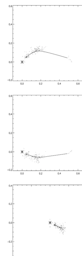
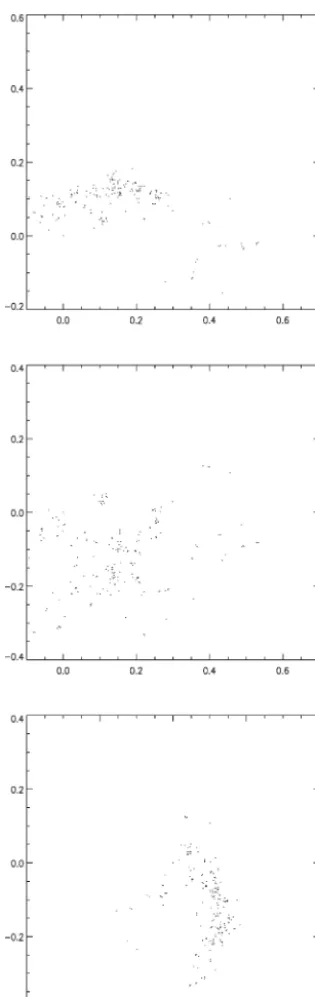
Figure 1.A view of the swarm (Stream 3, see Fig. 2) during the fitting process. We have overplotted the “default path” found for the swarm at that moment using the SOM algorithm. The projections (from top to bottom) are X–Yplane (orbital plane),X–Zplane andY–Zplane.

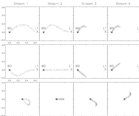
Figure 2.The four synthetic streams used to test the method. The different columns represent different streams, whilst the different rows show different projections (from top to bottom:X–Yplane,X–Zplane andY–Zplane, whereX–Yis the orbital plane and theXaxis points from the white dwarf towards the L1 point).

The fitting consists of minimizing a merit functionFby evolving the swarm shapes. The merit functionFis defined by

F=

n

i=1

Di−Mi

σi 2

+λSreg, (2)

where the first part is the normalχ2 _{part of the fit (D}

i are the data points,Mi the corresponding model values andσi the errors on the data points),λ is the Lagrangian multiplier and Sreg is a regularization term as described above (and in Appendix A). Our GA minimization is carried out using typically 500 different swarms per generation of solutions, and the convergence occurs typically in 50–100 generations. Note that whilst GA is used to minimize equation (2), the SOM algorithm is needed for evaluation of the regularization term (Sreg).

Fig. 1 shows an interim view of a swarm during the fitting process, as well as the current regularization curve for that particular swarm.

3 T E S T I N G T H E A L G O R I T H M

3.1 Model fits to synthetic data

Given the nature of the model and the fitting method, there is probably no formal way of proving the uniqueness of the

so-lutions. We therefore need to examine the method numerically, using synthetic data sets for which we know the shapes and locations of the emission regions (synthetic swarms). Here we present four such data sets and the corresponding results from our inversion.

In Fig. 2 we have plotted these data sets in three panels, showing theX–Y,X–ZandY–Zprojections of the data sets. The white dwarf is located at (0, 0, 0), and the centre of the secondary star at (1, 0, 0). Points with positiveZcoordinates are on the same side of the orbital plane as the observer for inclinations<90◦. The free-fall ballistic stream has a positiveYcoordinate.

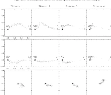
Then, given the four synthetic streams, we have computed four synthetic eclipse profiles, to which we have added noise (2 per cent RMS). These profiles, with corresponding model fits (generated using the GA and regularization described above) can be found in Fig. 3. The stream structures (swarms) producing these fits are plotted in Fig. 4: these can be directly compared with the original streams in Fig. 2.

We first consider the reconstructions in theX–Yplane. The syn-thetic streams have been reproduced remarkably well, with only very few points being wrongly attributed to the ballistic portion of the stream in the case of a wholly magnetically channelled stream (streams 3 and 4). In the case of theX–ZandY–Zplanes, we do not expect the reconstructions to be as good because at

3D eclipse mapping in AM Herculis systems

993

Figure 3.The fits to the synthetic data. The four fits correspond to the four test sets plotted in Fig. 2.

Figure 4.The best-fit reconstructions of the synthetic streams shown in Fig. 2. The panels are the same as in Fig. 2.

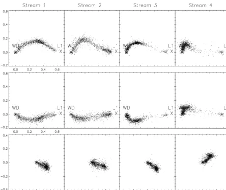
Figure 5.The results of 10 different reconstructions of the four test sets (see text for details). The different solutions are overplotted in each panel to demonstrate the stability of our solutions. The panels are the same as in Fig. 2.

an inclination of 80◦ (as used here) the eclipse profiles are dom-inated by movement in theX–Y plane. Nevertheless, the agree-ment is sufficient to be encouraging and the method is capable of discriminating between lower-pole and upper-pole accretion modes.

As the regularization term will force the ends of the stream to-wards the white dwarf and the L1 point, the resulting streams are also ‘rounded’ to some extent. In this sense the regularization acts somewhat like a rubber band, fixed to the white dwarf and L1 point at the ends and forced to pass through the swarm defining the stream.

3.2 Stability of the solutions

Secondly, we have studied the stability of our solutions, i.e. whether the resulting swarms always have the same location and shape. This is very easily done with our GA optimization code, as one only needs to start the fitting procedure with a different seed for the random number generator. This naturally leads to different initial swarm populations and thus we start at different locations in the parameter space. We have done this by fitting each of the synthetic data sets 10 times. The results can be seen in Fig. 5, where we have plotted the resulting 10 streams on top of each other. This figure, again, is directly comparable with Figs 2 and 4. Clearly all the solutions

are comparable with each other. Thus we believe that our method is capable of producing unique solutions.

3.3 Fits without the regularization term

To illustrate the effect of the regularization, we have carried out similar fitting without any regularization. For this purpose we have used Stream #3, a case where the ballistic part of the stream does not emit. As expected, the algorithm finds a perfectly adequate fit to the data (not shown), but the stream from this fit (Fig. 6) is a less faithful reproduction of the original stream (in Fig. 2). We can see that theX–Ylocations are reproduced to a fair extent, but theZ

direction is less well reproduced.

Fits without the regularization term are nevertheless extremely interesting – since even when the quasi-linear structure preju-dice for the stream is dropped, these fits represent the ‘minimum-assumption’ fits to the data. Multiple fits with different seeds, as used in Fig. 7, will indicate where emission from the stream could emanate, while remaining consistent with the data, and where it cannot.

We have therefore perfomed 200 fits without any regularization for Stream #3. The resulting ‘fly densities’ are shown in Fig. 7. One can clearly see that the main effect of the regularization term is that it controls the distribution of flies in theZplane. This is fairly natural

3D eclipse mapping in AM Herculis systems

995

Figure 6.The reconstruction of the third synthetic stream with no regular-ization. The panels are the same as in earlier figures.

since there is less information about theZcoordinate in the eclipse profiles.

3.4 Fixed parameters

In addition to the location of the fireflies, there are fixed parameters in our modelling which will, in principal, affect our results. We discuss these in more detail.

3.4.1 Effects of inclination

The system inclination and mass ratioq=M2/M1are not, in gen-eral, precisely known for all eclipsing systems. However, since we

Figure 7.200 reconstructions of the third synthetic stream with no regular-ization. This plot shows the resulting ‘fly density image’ in gray-scale. Note, that here the scale is larger covering most of the primary Roche lobe. The white dwarf is located always in the centre (marked by a diamond). Also the L1 point is marked similarly.XandYaxis labelling indicate the pixel resolution used for binning of flies. The panels are the same as earlier.

know the orbital period and the eclipse duration, the mass ratio is a function of inclination only. So it is sufficient to study how the results depend on using incorrect fixed inclinations for the modelling.

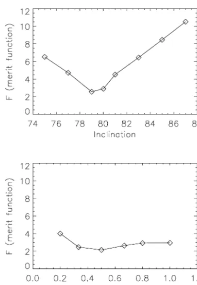
As earlier, we have used our synthetic Stream #3 as a testbed for our simulations. This set has an inclination of 80◦. We proceed to fit the corresponding eclipse profile with 8 different inclination values (fixed during each fit) ranging from 75 to 87◦. The results are plotted in Fig. 8 (top panel). Clearly, by fitting eclipse profiles using different inclinations, the change in merit function allows the inclination to be constrained by the fitting procedure.

Figure 8.The minimum values found for the merit function at given fixed inclinations (top) and fixed emissivity ratios (bottom). This was obtained using test Stream #3, which has a known inclination of 80 degrees and individual fly emissivity ratio of 0.5.

We could leave the inclination as a free parameter in our fits. However, its nature is different from the other fitted parameters (the three degrees of freedom per firefly), and this would require a some-what different fitting procedure. As it is known for some systems, we have opted to leave inclination as a fixed input parameter.

3.4.2 Effects of angular emissivity function

Secondly, we have studied the effect of the choice of emission law (equation 1). As in the case of inclination above, we have fitted Stream #3, which was created withF0=3.0,A=1.0 (white dwarf side twice as bright as the other side, emissivity ratio=0.5), with various values corresponding to the emissivity ratios (ER) of 0.2 to 1.0. Surprisingly, there was no significant difference in the quality of the fits, with the exception of ER=0.2, which gave a somewhat poorer fit. A plot of merit function versus fixed emissivity ratio is shown in Fig. 8 (lower panel).

The case of an optically-thin stream (and no X-ray heating, ER=1.0) produced a good fit, and the resulting stream structure is almost unchanged from theF0=3.0,A=1.0, ER=0.5 case. The implication is that, unless the emissivity function is known, a range of emissivity ratios must be explored to separate out the apparent as opposed to the angle-independent brightness of the stream. On the other hand, the choice of the ‘wrong’ emission law mainly leads to poorer fits, but the resulting stream structure is still very much like the one obtained using the correct emission law. This may be a consequence of the relatively narrow orbital phase range (∼40◦) used in our fits (e.g. the emission law would play a more significant

role in a case where one would try to fit whole light curves of these systems).

3.5 Single-pole versus two-pole emission

It is known, that some polars only accrete on to a single pole, whilst others accrete onto both poles (Cropper 1990). Some systems can even switch between single- and two-pole accretion modes. Thus it is worthwhile considering the effect of this on our modelling.

As our regularization term favours solutions where the accre-tion stream consists of single-line or curve-like structure, it is clear that such regularization cannot be correct for two-pole emission, in which the stream divides. In order to model two-pole accretion, we have experimented with regularization lines that, instead of starting from L1 and ending on a white dwarf, will both start AND end on the white dwarf. This would mimic a closed magnetic loop from one pole to another and, in theory, would enable us to find the most probable magnetic-loop-like emitting stream. However, tests with such synthetic streams did not prove very successful, and thus we have to limit our modelling to the single-pole accretion case for the time being. Further work on the regularization approach is needed to study this in depth.

4 C O N C L U S I O N S

We have presented a novel method to map the three-dimensional accretion-stream structure in eclipsing AM Herculis systems. Our approach is the first in which no a priori information is assumed about the trajectory of the accretion stream. This is important, as it allows us to study the possible changes in accretion-stream trajec-tory and accretion-region location at different epochs, in different accretion states and in different systems. Furthermore, by deter-mining the trajectory we will gain insight into the location of the magnetospheric threading region, and especially its distance from the white dwarf. This information, together with some assumptions of the stream density obtainable from the observations of X-ray dips (Watson et al. 1989), could provide us with more evidence on the accretion rate.

Our tests show that the inversion method is sufficiently robust to be applied to real data. This will be the subject of a forthcoming paper.

AC K N OW L E D G M E N T S

PJH is an Academy of Finland Research Fellow.

R E F E R E N C E S

Charbonneau P., 1995, ApJS, 101, 309 Cropper M. S., 1990, Sp. Sci. Rev., 54, 195 Hakala P. J., 1995, A&A, 296, 164

Hakala P. J., Watson M. G., Vilhu O., Hassall B. J. M., Kellett B. J., Mason K. O., Piirola V., 1993, MNRAS, 263, 61

Harrop-Allin M. K., Hakala P. J., Cropper M. S., 1999, MNRAS, 302, 362 Kohonen T., 1990, Proc. IEEE, 78, 1464

Kube J., G¨ansicke B., Beuermann K., 2000, A&A, 356, 490 Potter S. B., Hakala P. J., Cropper M. S., 1998, MNRAS, 297, 1261 Schwope A., Thomas H.-C., Beuermann K., 1993, A&A, 271, L25 Vrielmann S., Schwope A., 2001, MNRAS, 322, 269

Watson M. G., King A., Jones M. H., Motch C., 1989, MNRAS, 237, 299

3D eclipse mapping in AM Herculis systems

997

A P P E N D I X A : R E G U L A R I Z AT I O N U S I N G S E L F - O R G A N I Z I N G M A P S

Selforganizing maps (SOM) are a type of unsupervised neural net-works (Kohonen 1990). Their main use is data mining and cluster analysis of multidimensional data. Due to their topology conserv-ing nature, they can also be used to measure similarities within data samples. In our approach we have used them to find a best-fit curve through any given swarm of fireflies, which is then used as a ref-erence for computing the regularization function for that particular swarm (i.e. we find a smooth line through the swarm using SOM and compute the distances of individual flies to this line).

SOMs consist of a grid of ‘neurons’, which in the general case could beN-dimensional, but in our case it is one-dimensional. Each of the neurons has a set of weights associated with it. The number of weights per neuron is exactly the same as the dimensionality of the input data (in our case this means that the SOM ‘net’ consists of 20 neurons (defining the smooth line) and each neuron has three weights, which are simply itsX Y Z coordinates).

In a trained network, these weights will directly define the coor-dinates of the cluster centre associated with that particular neuron (i.e. the location of the neuron in data space). To start with, these weights can have either random values or they can span some pre-defined space otherwise. Here we chose to initialize the weights by placing the neurons equidistantly along the line from white dwarf to the L1 point.

A1 Training SOMs

The training of the network proceeds as follows. First a random data pointPis chosen from the training sample of data points, in our case this would mean a selection of a random firefly from a swarm. Next, one computes for each neuronNi, that has a set ofjweights

Di = P−Ni,∀i, (A1)

i.e. the euclidean distance between the sample data pointP(single firefly) and the neuronNi. Then we define the winning neuronNw

as the one that has minimumDi i.e. is the closest one to the input pointP(chosen firefly).

Next, the network is trained. This means simply, that for any given swarm: We select a random fly, find the nearest neuron to it in 3D space (A1), move that neuron (and it’s neighbouring neurons as defined below) towards the location of that fly (A2), and then proceed to the next random fly from our swarm. This is iterated for about 5000 times (every fly gets selected on the average about 25 times) and as a result the neurons define a smooth curve through the swarm.

Formally this happens as follows:

Ni(t+1)=Ni(t)+h(i, w)[P−Ni(t)],∀i, (A2)

whereNi(t+1) is the updated neuron weight vector andh(i, w) is a neighbourhood kernel, which depends on the distance of neuron

Nifrom the winning neuronNwin the following manner:

h(i, w)=α(t)e

−r_i−rw2

2σ(t)2 ,∀_i. _(A3)

Here,α(t) is a time dependant learning rate,ri−rw2is the squared

distance between the winning NeuronNw and the current neuron to be trainedNi. Note that this distance is the distance between the two neurons on the grid, and not the distance between their weights.

σ(t) is the time dependent width of the kernel. Other forms than

the Gaussian dependance forh(i, w) are also possible. The effect of the neighbourhood kernel is that whilst the weights of the winning neuron are moved towards the input data also the weights of its neighbouring neurons (on the grid) are moved, but with smaller amount. This ensures the topology conserving mapping, typical to the SOM.

This completes one training step. Next one selects a new random input and iterates again. The learning rateα(t) and the kernel width

σ(t) are both constantly lowered during the training.

A2 Application to regularization

As a result of training, the SOM will find a predefined number of clusters in the input data. For our purposes we are not really interested in the clustering, but use the SOM to find a predefined ordered set of nodes that define a smooth curve through our swarm of fireflies. This is achieved by training a one-dimensional SOM with fireflies as input points. In addition, about 20–30 per cent of the input points are not fireflies but contain either the coordinates of the white dwarf or the L1 point. We also give a constraint that the ‘white dwarf points’ should be mapped to the other end of the map and the ‘L1 points’ to the other. This then produces a curve that stretches from near the L1 point, through the swarm and terminates near the white dwarf.

The regularization itself means that we prefer solutions that are well represented with the curve computed as above. Formally, we use a SOM with 20 neurons, weights of which originally span the distance from the L1 point to the white dwarf equally spaced. Af-ter training the net with about 5000 inputs randomly selected as explained earlier, we have the default path defined for the given swarm. We now compute the regularization termSregas a sum of squared distances from this default path for all our 200 fireflies:

Sreg= 200

k=1

(Pk−Nw,k)2. (A4)

HerePkis a vector in 3D space representing the location of a single

firefly and Nw_,kis the location of the nearest (to the Pk) neuron.

This type of regularization prefers solutions that are ‘stream-like’ with fixed ends, but leave the stream path totally free.

A P P E N D I X B : G E N E T I C O P T I M I Z AT I O N

The Genetic Algorithm (GA) used here for optimization is simi-lar to those used in Hakala (1995); Harrop-Allin et al. (1999) and Potter et al. (1998). There are, however, some alterations specific to this procedure. In our current approach the ‘genes’ that define the solution swarm are the locations of the individual fireflies.

In general, the algorithm proceeds as follows. First we create a a population of∼500 random solutions i.e. 500 random swarms inside the Roche lobe of the primary. Secondly, we evaluate these solutions. Next, we select the parent solutions to produce offspring. This is done by first selecting five random solutions, the fittest of which is chosen as 1 parent. This is repeated to choose the second parent. Two offspring solutions are produced by ‘mixing’ the parent swarms. In practice this is done by picking fireflies at random from the two parent swarms. Offspring solutions are mutated in three different ways. First, at a small probability of∼0.002 any firefly within the swarm can be removed and replaced by a new random firefly. With slightly higher probability, a firefly can be mutated by changing its location by a small gaussian random number. Finally a small fraction (∼5 per cent) of the fireflies in the resulting swarm

are mutated by moving them slightly towards the regularization curve for that particular swarm (computed using the SOM method as explained above). This speeds up the process when it otherwise gets very inefficient towards the latter stages of fitting.

Having created offspring solutions we then evaluate them and if they are better than their parent solutions they will replace the

parents in the population. This procedure is repeated until some predefined convergence criterium is achieved or some fixed number of generations has passed.

This paper has been typeset from a TEX/LA_{TEX file prepared by the author.}