A Complementary Heuristic for the Unbounded
Knapsack Problem
Swarna Chitra Iyer
A thesis submitted in fulfilment of the requirements for the
Masters' degree
Department of Computer and Mathematical Sciences
Victoria University of Technology
Declaration
I hereby certify that:
1. the following thesis contains only m y original work,
2. due acknowledgment has been made in the text of the thesis to
all other material used and
3. the thesis is less than 60,000 words in length, exclusive of tables,
figures and footnotes.
Swarna Chitra Iyer
ABSTRACT
A s a solution algorithm for U n b o u n d e d Knapsack Problem, the
performance analysis of density-ordered greedy heuristic, weight-ordered
greedy heuristic, value-ordered greedy heuristic, extended greedy
heuristic and total-value heuristic has been done. Empirical experiments
o n different test problems have been analysed and reported. Problem
instances with a very large n u m b e r of undominated items were generated
in addition to the types of instances suggested by Martello and Toth
(1990). Theoretically, the lower b o u n d o n the performance for total-value
heuristic is better than the corresponding lower bounds for the
density-ordered greedy heuristic and the extended greedy heuristic as discussed
by White (1992) and Kohli and Krishnamurti (1992). T h e computational
tests fail to s h o w clear superiority of any particular heuristic algorithm,
although each heuristic produces good quality solutions. If the
combination of the density-ordered greedy and the total-value greedy
heuristics are considered then the combination s h o w s complementary
effect. A n e w heuristic algorithm incorporating the structural properties of
the density-ordered greedy heuristic and the total-value greedy heuristic
is developed and its complementary effect studied. It w a s found that the
combination of the density-ordered greedy heuristic, the extended greedy
heuristic, the total-value greedy heuristic and the n e w complementary
heuristic gives a better performance result than the single best heuristic in
Acknowledgments
I would like to thank:
• m y parents, Sharada and Subramanian
• m y supervisor, Lutfar Khan
• m y colleagues, particularly M e h m e t Tat, Tony Sahama, and D a m o n
Burgess and P. Rajendran (Raj) for their technical support,
CONTENTS
List of Figures viii
List of Tables ix
1 Fundamentals 1
1.1 Knapsack Problems and its Variants 1
1.1.10-1 Knapsack Problem 3
1.1.2 Unbounded Knapsack Problem 3
1.1.3 Bounded Knapsack Problem 3
1.2 Objective of Study 5
1.3 Organisation of the Thesis 6
2 Literature Review 7
2.1 Exact Versus Heuristic Algorithms 7
2.2 Solution Algorithm for Knapsack Problems 9
2.2.1 0-1 Knapsack Problem 9
2.2.2 Bounded Knapsack Problem 10
2.2.3 Unbounded Knapsack Problem 10
2.3 Heuristic Algorithms for the Unbounded Knapsack
Problem 11
2.3.1 Density-ordered Greedy Heuristic 11
2.3.2 Weight-ordered Greedy Heuristic 13
2.3.3 Value-ordered Greedy Heuristic 14
2.3.4 Extended Greedy Heuristic 15
2.3.5 Total-value Greedy Heuristic 16
2.3.6 Combination of Greedy Heuristics 19
2.4 Meta-Heuristics 20
2.4.1 Simulated Annealing 21
2.4.2 Tabu Search 22
2.4.3 Genetic Algorithms 23
2.5 Martello-Toth Exact Algorithm 26
2.6 Dominance Criteria 28
3. Empirical Analysis of Heuristics for the Unbounded Knapsack
Problem 30
3.1 Computational Design and Data Generation 30
3.2 Effect of Dominance on the Five Problem Classes 33
3.3 Performance Measures and Factors 36
3.3.1 Measuring Performance 36
3.3.2 Factors that Influence the Performance of a Heuristic
Algorithm 38
3.4 Results 38
3.5 Analysis of the Results 53
4. Complementary Effect of Heuristics 61
4.1 Comparison of Heuristics 61
4.2 Complementary Total-value Greedy Heuristic 63
5. Summary and Conclusion 72
5.1 S u m m a r y 72
5.2 Conclusion 74
5.3 Further Scope for Research 75
Appendix 76
Appendix A: F O R T R A N Codes for Data Generation 76
Appendix B: F O R T R A N Implementations of the Heuristic 80
Algorithms
Appendix C: Analysis of Different Ratio Ranges in the
Appendix D: Difficult Instances of the Unbounded
Knapsack Problem 99
REFERENCES 105
List of Figures
3.1a N u m b e r of undominated items for Uncorrelated,
Weakly Correlated and Strongly Correlated Class of U K P 35
3.1b N u m b e r of undominated items for Very Strongly
and Very Very Strongly Correlated Class of U K P 35
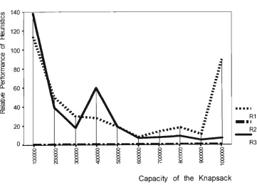
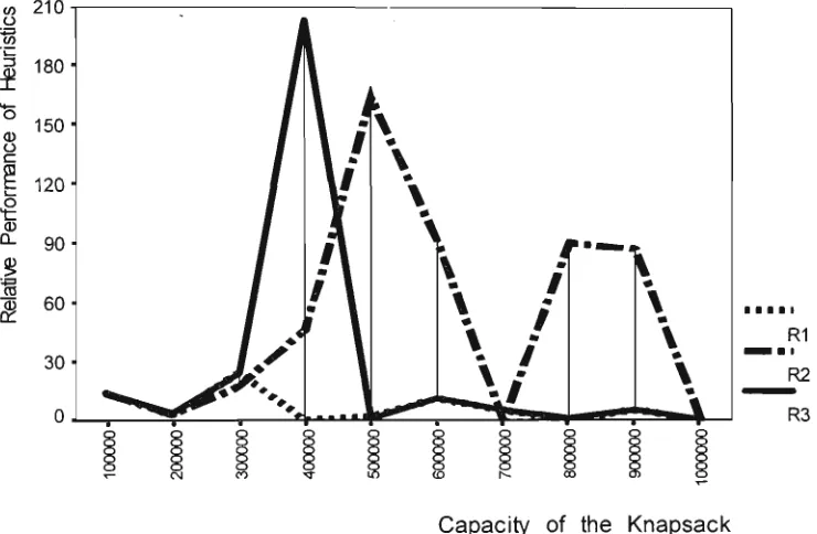
3.2 Very Strongly Correlated Class (Class IV), n = 50 53
3.3 Very Strongly Correlated Class (Class IV), n = 100 54
3.4 Very Strongly Correlated Class (Class IV), n = 500 54
3.5 Very Strongly Correlated Class (Class IV), n = 1000 55
3.6 Very Strongly Correlated Class (Class IV), n = 5000 55
3.7 Very Strongly Correlated Class (Class IV), n = 10000 56
3.8 Very Strongly Correlated Class (Class IV), n = 20000 56
3.9 Very Strongly Correlated Class (Class IV), n = 30000 57
3.10 Very Strongly Correlated Class (Class IV), n = 40000 57
3.11 Very Strongly Correlated Class (Class IV), n = 50000 58
3.12 Very Very Strongly Correlated Class (Class V), n = 100 59
3.13 Very Very Strongly Correlated Class (Class V), n = 500 60
CI Ratio range [5.0,5.2] 97
List of Tables
2.1 Worst-case bounds for the density-ordered greedy
heuristic and the total-value greedy heuristic 18
3.1 Sample data sets for the five problem classes 32
3.2 Average n u m b e r of undominated items (average of 5
problem instances for each class and each n) 34
3.3 Comparison of solutions for Hi, A and B (for the five
problem classes, 500 problem instances in each class) 40
3.4(a&b)Computational results for the uncorrelated class
(Class I) of problems 43,44
3.5(a&b)Computational results for the weakly correlated
class (Class IT) of problems 45,46
3.6(a&b)Computational results for the strongly correlated
class (Class III) of problems 47,48
3.7(a&b)Computational results for the very strongly correlated
class (Class IV) of problems 49,50
3.8(a&b)Computational results for the very very strongly
correlated class (Class V) of problems 51, 52
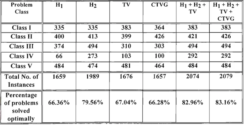
4.1 N u m b e r of instances where the heuristics give optimal
solution; 500 instances in each case 62
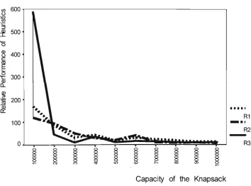
4.2 Comparison of solutions for C T V G , H i and T V
for the Class I problems; 50 instances in each r o w
(5 data sets and 10 different capacities) 67
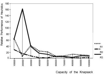
4.3 Comparison of solutions for C T V G , H i and T V
for the Class II problems; 50 instances in each r o w
(5 data sets and 10 different capacities) 67
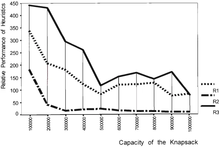
4.4 Comparison of solutions for C T V G , H i and T V
for the Class III problems; 50 instances in each r o w
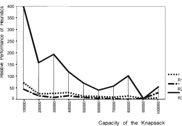
.5 Comparison of solutions for C T V G , Hi and T V
for the Class IV problems; 50 instances in each row
(5 data sets and 10 different capacities)
4.6 Comparison of solutions for C T V G , Hi and T V
for the Class V problems; 50 instances in each row
(5 data sets and 10 different capacities)
4.7 N u m b e r of instances where the heuristics give
optimal solution; 500 instances in each case
CI Average no. of undominated items for
different ratio ranges: total no. of items
considered is 10000
D l Computational results for n = 100, 200, 300,
CHAPTER 1
1. FUNDAMENTALS
Knapsack problems are intensively studied mainly for their simple
structure which, on the one hand allows exploitation of a number of
combinatorial properties and, on the other, facilitates the solution of more
complex optimisation problems through a series of knapsack-type
subproblems.
In the following sections we shall examine in brief, the most common
variants of Knapsack Problems and outline the design of this thesis.
1.1 Knapsack Problems and its Variants
A typical investment problem can be described as follows.
Given an amount of investment capital, a variety of projects with different
capital requirements and expected profits are possible. Some of the
projects are to be selected such that the budget is not exceeded and the
total expected profit is maximum.
This decision problem is an important application model of the Knapsack
Problem (KP).
The name Knapsack Problem comes from its relation to the hitch-hiker's
decision making situation (which is the same as the investment example);
a hitch-hiker packs his knapsack by selecting from among various possible
objects those which will give him m a x i m u m utility or profit without
Mathematical programming problems like Linear Programming and Integer
Programming have been applied in a number of decision making
situations. A K P can be classified as an integer programming problem.
Because of its combinatorial structure, it is often treated as a combinatorial
optimisation problem.
Mathematically, a KP can be formulated as:
Given a set of n items and a knapsack, with
pj = profit (or value) of item j, Wj = weight (or volume) of item j,
C = capacity of the knapsack,
select a subset of the items so as to
n
Maximise z = '^_lpjxJ
y=i
n
subject to ^,wjxj - C
Xj = 0 or 1, j e N = {1,2, ... ,n}
where Xj = 1, if item j is selected;
= 0, otherwise.
In the literature this one-constraint, linear pure 0-1 discrete programming
problem is called the 0-1 Knapsack Problem or simply the Knapsack
Problem. It is also k n o w n as the Lorie-Savage Problem (1955).
There are different variants of the Knapsack Problem, some are described
in the following.
.. (1)
.. (2)
1.1.1 0-1 Knapsack Problem
The problem defined by equations (1), (2), & (3) is called the 0 - 1
Knapsack Problem (0-1 KP). The term 0-1 appears because an item is
either selected or rejected, and at most one piece of each item can
be selected.
1.1.2 Unbounded Knapsack Problem
W h e n it is possible to select any number of pieces of an item, the problem
is called an Unbounded Knapsack Problem (UKP),
i.e., w h e n equation (3) is replaced by
Xj > 0, integer (4)
where Xj = number of units of item j selected, then U K P is the
problem defined by equations (1), (2), & (4).
In this thesis, w e will be dealing with the solution algorithms for U K P .
1.1.3 Bounded Knapsack Problem
W h e n for each item there is an upper limit to the number of pieces that can
be selected, the problem is called a Bounded Knapsack Problem (BKP),
i.e., w h e n equation (4) is replaced by
0 < Xj < bj, j G N = {1,2, ... ,n} (5)
Xj integers,
then B K P is the problem defined by equations (1), (2), & (5).
Strictly speaking, an U K P is a special case of BKP, since replacing bj by oo
or a value defined by the knapsack capacity and Wj, they are equivalent.
The 0 - 1 KP, UKP and BKP are generally referred to as Knapsack
Problems (KP). KPs have been intensively studied as discrete
programming problems. The reason for such interest basically derives
(a) a K P can be viewed as one of the simplest Integer Programming
problems;
(b) it appears as a subproblem in complex problems as in cutting
stock problem. The solution of knapsack problems in solving
cutting stock problems (Gilmore and Gomory, 1963) is
particularly important because of the fact that in the column
generation procedure that is used for cutting stock problem,
repeated solution of Unbounded KnapsackProblems are used;
(c) it represents a great many practical situations such as capital
budgeting, project selection, loading problems, journal selection
in a library (Salkin and de Kluyver, 1975).
There are many other variants of KP and similarly structured
mathematical models. They can be classified under two categories.
The knapsack problems, where only one knapsack is to be filled with an
optimal subset of items are called Single Knapsack Problems. The 0-1
knapsack problem, the hounded and unbounded knapsack problems, the subset-sum problem, the change-making problem are all single knapsack problems.
The knapsack problems where more than one knapsack is available are
called Multiple Knapsack Problems. The 0-1 multiple knapsack problem, the
generalised assignment problem and the bin-packing problem can be called
multiple knapsack problems.
These problems are discussed in detail in Taha (1975), Salkin and Mathur
(1989) and Martello and Toth (1990); the last one includes computer codes
1.2 Objective of Study
Knapsack Problems (KP) are widely used mathematical decision models,
particularly in the areas of cutting stock, cargo loading, capital investment,
etc. K P and its variants are in the class of difficult optimisation problems,
which take u p long computational time. The particular variant of K P
studied in this research, namely the U n b o u n d e d Knapsack Problem
( U K P ) , w a s first introduced s o m e decades ago and the density-ordered
greedy heuristic algorithm has been available since. In the 1990s, a n e w
algorithm, called the total-value greedy heuristic appeared, but not fully
explored in terms of computational time and quality. A detailed report o n
the exact (optimal) solution algorithms w a s published only lately ( in
1990).
In this research all the available heuristic algorithms for UKP have been
studied. T h e aims of this research is to generate test problems and
investigate the performance of the algorithms in solving different
instances of these problems by varying parameters such as problem size,
knapsack capacity and profit/ weight ratios. In particular, an extensive
study of the performance of the density-ordered greedy heuristic, the
weight-ordered greedy heuristic, the value-weight-ordered greedy heuristic, the extended greedy heuristic and the total-value greedy heuristic are undertaken by comparing
the quality of their solutions and the computational time with respect to
the Martello-Toth exact algorithm. T h e results are expected to be useful in
developing algorithms and software in related areas. In the c o l u m n
generation technique for solving linear programming problems, the ease
of solving K P s will be helpful. Although, it has been the practice to take
the c o l u m n corresponding to the optimal solution of the K P , it is not
absolutely necessary to d o so. Gilmore and G o m o r y (1963) observed that
1.3 Organisation of the Thesis
Chapter 2 describes in brief the existing algorithms for the knapsack
problem. Algorithms for the variants of K P are outlined in Section 2.1 and
a detailed discussion of the solution algorithms for the u n b o u n d e d
knapsack problem is given in Section 2.2. Section 2.3 gives a brief
description of the meta-heuristics and their likely use in finding solutions
for knapsack and related problems. Section 2.4 explains Martello-Toth's
exact algorithm for U K P . Dominance criterion, an important p h e n o m e n o n
used to greatly reduce the size of the original problem is discussed in
Section 2.5. Chapter 3 is a detailed description of the computational
analysis of the heuristics for U K P . Section 3.1 describes the computational
design and data generation for the heuristics and gives a few sample
datasets for the five problem classes generated. Section 3.2 describes the
performance measures and the factors that are to be recognised in an
experimental study of heuristics. Section 3.3 and 3.5 reports the
computational results obtained o n the five heuristic algorithms for U K P .
Sections 4.1 describes the complementary effect of heuristics. Based o n the
behaviour of the existing heuristics, a n e w complementary heuristic is
developed and is discussed in Section 4.2. S u m m a r y and conclusion is
given in Chapter 5. The F O R T R A N codes for data generation are given in
Appendix A and the code for the heuristic algorithms is given in
Appendix B; in Appendix C, the effect of varying the density ratio range is
explained for the Class IV problem instances and in Appendix D s o m e
difficult problem instances of Class V U n b o u n d e d Knapsack Problem are
CHAPTER 2
2. LITERATURE REVIEW
The sections in this chapter describe the solution algorithms for Knapsack
Problem in brief and discusses the heuristic algorithms for the Unbounded
Knapsack Problem at length. The dominance criterion which is an
important phenomenon in any solution algorithm for U K P is described in
Section 2.5.
2.1 Exact Versus Heuristic Algorithms
The time-complexity or, simply, complexity of an algorithm for solving some
problem is said to be the maximal number of computational steps that it
takes to solve any instance of the considered problem of a given size. For
example, the time-complexity of a given algorithm as a function of the size
s is the order of f(s), w h e n s -» QO and is denoted by 0(i(s)) or simply
0(8).
An algorithm can be classified as good or bad depending on whether or
not it has polynomial time complexity. Similarly, a problem can be
classified as 'hard' or 'easy' depending on whether or not it can be solved
exactly by an algorithm with polynomial time complexity. Based on this
distinction, an elegant theory of the complexity of problems has been
developed (Garey and Johnson, 1979).
Mathematical decision problems can be grouped into two classes, viz.,
easily solvable problems (class P) for which polynomial algorithms are
k n o w n and problems which require considerable computing time (class
problem type is in the class P if there exists an algorithm that, for any
instance, has running time (the number of computational steps required)
that is bounded by a polynomial function of the problem size, i.e.,
problems for which polynoniial-time algorithms have been devised. A
problem type is in the class N P if it is possible to devise an algorithm for
each problem, but no polynomial-time algorithm is k n o w n for any of
them. For example, the problem of finding the maximal number among n
numbers requires n-1 comparisons, thus such a problem is in P. For a 0 -1
knapsack problem with n items to be solved exactly, w e have to check, in
the worst case, all 2n combinations of items. Such a problem is in NP.
A problem is termed NP-Complete if (i) it belongs to NP and (ii) it has a
property that if an efficient algorithm is found for it then an efficient
algorithm can be found for every problem in NP. In this sense the N P
-Complete problems are the hardest in NP. KPs are NP--Complete problems
(Garey and Johnson, 1979) and are difficult to solve optimally. Obviously,
the difficulty rises rapidly if the number of items go up.
An exact algorithm guarantees an optimal solution to a mathematical
progranvming problem. The two principal approaches for finding an
optimal solution to an integer-programming problem are the
branch-and-hound algorithm and the dynamic programming algorithm. Although there
are noticeable differences among different problems, in general the N P
-Complete problems require a lot of computational time.
Heuristic algorithms give near - optimal solutions in reasonably short
computational time. Heuristic solutions to different combinatorial
problems can be found using a number of heuristics. For a KP, the use of
a heuristic algorithm m a y be justified for several reasons. First, it is often
necessary and that one would be content with a solution that is sufficiently
close to the optimal. This m a y well be the case, for instance, w h e n the
profit pj, themselves are only estimates of expected returns or w h e n the
knapsack problem is only a sub-optimisation of a m u c h larger problem.
Further as w e see that there is no k n o w n polynomial algorithm for this
problem and that there m a y well not be any such algorithm, restrictions
on computing time m a y force one to be satisfied with a heuristic solution
to large problem instances.
Although this study deals with UKP, solution methods for very closely
related problems of 0 - 1 K P and B K P are briefly discussed in the
following.
2.2 Solution Algorithms for Knapsack Problems
Following the notation of complexity as 0(s), it can be said that for a
KP, s is the number of possible items. In the discussion below, n is the
number of items and C is the knapsack capacity.
2.2.1 0 -1 Knapsack Problem
This problem can be solved exactly by reduction algorithms where the
number of variables are first reduced before applying the algorithm
(Ingargiola and Korsh, 1973; Martello and Toth, 1988, 1990 and Nauss,
1996). It can also be solved heuristically by a method of relaxation and
upper bounds (Dantzig, 1957), where the computation for the Dantzig
bound requires 0(n) time if the items are sorted according to
non-increasing values of the profit per unit weight. Other heuristic algorithms by
0-1 K P include Sahni (1975) and Balas and Zemel (1980), which require
2.2.2 Bounded Knapsack Problem
This problem can be solved exactly by branch-and-bound algorithms
(Martello and Toth, 1977; Ingorgiola and Korsh, 1977 and Bulfin et al.,
1979). Aittoniemi and Oehlandt (1985) gives an experimental comparison
of these, indicating the Martello and Toth (1977) one as the most effective.
It can also be solved by dynamic programming (Gilmore and Gomory, 1966;
Nemhauser and Ullmann, 1969) method requiring 0(nC?) time in the
worst case and the space complexity is 0(nC) and can only solve problems
of very limited size. The heuristic solution algorithms are upper bounds and
approximate algorithms, where the computation time is 0(n).
2.2.3 Unbounded Knapsack Problem
The solutions to this problem include exact algorithms based on branch
-and - bound (Martello -and Toth, 1977; Cabot, 1970; Gilmore -and Gomory,
1963) and dynamic programming (Garfinkel and Nemhauser, 1972). The
heuristic algorithms are upper bounds and approximate algorithms (Magazine
et al, 1975; H u and Lenard, 1975), the time complexity for the computation
of the upper bounds is 0(n) and the time complexity of the approximate
(Greedy) algorithm is 0(n), plus 0(n log n) for the preliminary sorting.
This research focuses on the solution of the Unbounded Knapsack
Problem (UKP). In the literature, there are five main heuristic algorithms
for U K P :
a) Density - ordered greedy heuristic (Dantzig, 1957; Martello and Toth,
1990),
b) Weight - ordered greedy heuristic (Horowitz and Sahni, 1978; Kohli and
c) Value - ordered greedy heuristic (Horowitz and Sahni, 1978; Kohli and
Krishnamurti, 1995),
d) Extended greedy heuristic (White, 1991),
e) Total - value greedy heuristic (White, 1992; Kohli and Krishnamurti,
1992; Lai, 1993).
2.3 Heuristic Algorithms for the U n b o u n d e d K n a p s a c k Problems
The aforementioned five heuristic algorithms are discussed in the
following.
The solution method of these five greedy heuristics is termed 'greedy'
because at each step ( except possibly the last one ) w e choose to introduce
that object which according to one criterion or the other w o u l d increase
the objective function value the most. A n object once selected, stays in the
knapsack and therefore in the solution. The items can be ordered (a) in
decreasing order of density pi/wi, (b) in increasing order of the item
weights Wi, (c) in decreasing order of the profit of the item pi and (d) in
decreasing order of the total-value Lc/wi J pi.
2.3.1 Density - ordered Greedy Heuristic (HJ
This is the classic heuristic for the unbounded knapsack problem. This
procedure has been discussed in the literature a m o n g others, by Garey
and Johnson (1979) and Martello and Toth (1990). Dantzig (1957) first
Density-ordered greedy heuristic recursively determines a solution by
making a variable with smallest marginal unit cost as large as
possible.
First, order the items so that
pi > P2 > > pn-l > Pn
where, pj = PJ/WJ , 1 < j < n
Then set
(a) xi = L C / w J ;
(b) XJ = L(C - f>,wj/wjj , 2<j<n
k=\
where for z e Z+ , |_zj is the integer part of z.
Hi gives good results, but the worst case result is poor and it can be
shown that there are instances where the optimal solution is almost twice
the greedy solution. Under some restrictive assumptions, the greedy
algorithm will give optimal solution (Magazine et al, 1975; H u and
Lenard, 1975; White, 1991). A n example of Hi is as follows.
Example 1
C = 100
W 2 = 50, wi = 51
p2 = 99, pi = 102
pi = 102/51 > p2 = 99/50
Hi -> x2 = 0, xi = 1, z(Hi) = 102
Optimal -> x2 = 2, xi = 0, z(opt) =198
The heuristic solution value is almost half of the optimal solution value.
2.3.2 Weight - ordered Greedy Heuristic (A)
Horowitz and Sahni (1978) formulated a greedy approach attempting to
obtain a solution. This method tries to be greedy with the capacity and
thus requires the objects to be ordered in non-decreasing weights, w e try
to put as m a n y objects as possible with the least weight into the knapsack,
thus using up as m u c h capacity. This heuristic has arbitrarily bad
worst-case bounds (Horowitz and Sahni, 1978; Kohli and Krishnamurti, 1995)
though the capacity is used up slowly with the profits coming in rapidly
enough. Example 2 shows a very bad instance for Heuristic A.
Example 2
C = 100
W 2 = 10, wi = 9
p2 =1000, pi = 1
A -> x2 = 0, xi = 11
z(A) = 11
Optimal -> X2 = 10, xi = 0
z(opt) = 10000
z(A) = 0.0011 z(opt)
It is possible to find randomly generated instances where the
weight-ordered greedy heuristic provides the optimal solution value (Example 3).
In general they are expected to perform poorly.
Example 3 C = 20
W3 = 10, W 2 = 15, wi = 18 p3 = 15, p2 = 24, pi = 25
A -> x3 = 2, x2 = 0, xi = 0
Optimal -> x3 = 2, x2 = 0, xi = 0, z(opt) = 30
2.3.3 Value - ordered Greedy Heuristic (B)
This greedy heuristic discussed by Horowitz and Sahni (1978) followed
by Kohli and Krishnamurti (1995) considers objects in order of
non-increasing profit values. This method too has arbitrarily bad worst-case
bounds (Horowitz and Sahni, 1978; Kohli and Krishnamurti, 1995) and
does not usually yield an optimal solution though the objective function
value takes large increases at each step. The number of steps is reduced as
the knapsack capacity is used up at a rapid rate. A bad instance is given in
Example 4.
Example 4
C = 100
W 2 = 99, wi = 1
P2 = 2, pi = 1
B -> X2 = 1, xi = 1
z(B) = 3
Optimal -> x2 = 0, xi = 100
z(opt) = 100
z(B) = 0.03 z(opt)
There are of course instances where the value-ordered greedy heuristic
gives the optimal solution value (e.g., Example 5). In general, this heuristic
too is expected to perform poorly.
Example 5 C = 80
p4 =36, p3 =20, p2 =20, pi = 9
B -> X4 = 4, x3 = 0, x2 = 0, xi = 0, z(B) = 144
Optimal -^ X4 = 4, X3 = 0, X2 = 0, xi = 0, z(opt) = 144
2.3.4 Extended Greedy Heuristic (H2)
White (1991) discussed an extension of Hi, which he called H2. This
involves pairs of items rather than a single item as in the density-ordered
greedy heuristic. It requires that the best combination of the first two
items (from the ratio sorted list in non - increasing order) be taken and
then the best combination of the next two items is taken, and so on.
Unfortunately, neither H 2 is always superior to Hi nor indeed is Hi always
superior to H2. Although the worst case result with a ratio bound of 2 is
the same for both heuristics, on many occasions the two-at-a-time heuristic
(H2) can be better. It is possible that Hi gives an optimal solution, with H 2
not giving an optimal solution and also it is possible that H 2 gives an
optimal solution, but Hi does not give an optimal solution. If Hi uses up
exactly the available resources, then Hi definitely gives the optimal
solution. But this need not be true with H2. Example 6 is an instance where
H 2 is better than Hi.
Example 6
C = 10
W3 = 3, W 2 = 2, Wl = 1
p3 = 14, p2 = 8, pi = 1
p3 = 14/3 > p2 = 4 > pi = 1
Hi -> x3 = 3, x2 = 0, xi = 1, z(Hi) = 43
Example 7 is an instance where H 2 is worse than Hi.
Example 7
C = 10
W4 = 3 , W3 = 2, W2 = 1, Wl = 1
P4 = 20, p3 = 12, p2 = 5, pi = 1
p4 = 20/3 > p3 = 6 > p2 = 5 > p i = l
Hi -» X4 = 3, X3 = 0, X2 = 1, xi = 0, z(Hi) = 65
H2 -> x4 = 2, x3 = 2, x2 = 0, xi = 0, z(H2) = 64
If combinations of 3 or more items are considered instead of 2, w e
might call them H3, H4, and so on. These, however, clearly increases
computation time requirements and lose the benefits of obtaining
solutions quickly. It m a y be noted that Hn, where n = number of items, is
in fact an exact algorithm for the original problem.
2.3.5 Total-Value Greedy Heuristic (TV)
Total-Value Heuristic (White, 1992; Kohli and Krishnamurti, 1992; Lai,
1993) is another heuristic solution method for the unbounded knapsack
problem.
At step i, the total-value heuristic selects an item for which the values
PJ LCI/WJJ across all available items j is maximum, where Ci is the
available knapsack capacity at the beginning of step i. The items need
not be sorted in a non-increasing order, because all the items have to
Example 8 is an instance where the total-value greedy heuristic gives the
optimal solution value. The density-ordered greedy heuristic and the
extended greedy heuristic in this instance performs poorly.
Example 8
C = 30
W4 = 12, W3 = 10, W2 = 9, Wl = 8
p4 = 22, p3 = 21, p2 = 20, pi = 19
p4 = 22/12 < p3 = 21/10 < p2 = 20/9 < pi = 19/8
Hi -> X4 = 0, x3 = 0, x2 = 0, xi = 1, z(Hi) = 57
H2 -> x4 = 0, x3 = 0, x2 = 2, xi = 1, z(H2) = 59
T V -» x4 = 0, x3 = 3, x2 = 0, xi = 0, z(TV) = 63
Optimal -» X4 = 0, X3 = 3, X2 = 0, xi = 0, z(opt) =63
Lai (1993) called this solution method as Heuristic A. He showed that this
heuristic has a worst-case performance ratio > 4/7.
White (1992) and independently Kohli and Krishnamurti (1992) showed
CO
that the worst case bound of T V given by 1/ ]JT 1 / h(i) where h(i ) is an
integer value given by the recursion h(l) = 1, h(2) = k + 1, h(i ) = [h(i
-1)].[h(i - 1)+1] for i > 3, is always better than that of Hi given by k/(k
+ 1) (Fisher, 1980) where k is the integer part of the ratio of the
knapsack capacity to the weight of the heaviest item, i.e., k =
LC/wmaxJ. Hi behaves like T V with the integrality constraint removed
(i.e., if the fractional amounts of items are allowed to be included in the
knapsack). The performance of the heuristics depend on k. A s k
increases, the difference between Ll/wJ and 1/wi for i = 1, 2, ..., n is
tends to be the ordering d u e to the density-ordered greedy heuristic. A s a
result the difference between the t w o worst-case bounds decreases.
The principal benefit of the total - value heuristic appears to be in the fact
that it considers all three parameters — unit weight, unit value and
knapsack capacity — in ordering items, i.e., it selects items in a
non-increasing order of their m a x i m u m possible contribution to the solution
value given the available knapsack capacity at each step. A consequence of
considering all three parameters is that T V always gives a better worst-case
performance than that of Hi for the unbounded knapsack problem as s h o w n
in Table 2.1. Individual problem instances d o however exist where H i
gives better results than T V (e.g., Example 9).
Table 2.1: Worst-case Bounds for Density - ordered Greedy Heuristic and Total-value Heuristic. Q7rom Kohli & Krishnamurti, 1992)
t k 1 2 3 4 5
r(TV) 0.5913555 0.7026825 0.7678212 0.8101038 0.8396093
r(Hi) 0.5000000 0.6666667 0.7500000 0.8000000 0.8333333
W e observe from the above table that the difference between the
worst-case b o u n d for T V and H i is the largest for k=l. This difference decreases
as k increases. A s k approaches infinity, both heuristics obtain the optimal
solution. Because of the greater n u m b e r of operations needed per step, T V
takes m o r e computational time than Hi.
t k = n u m b e r of the largest item that can fit into the knapsack and
Example 9
C = 41
W 7 = 7 , W6 = 8, W5 = 5, W 4 = 4, W3 = 9, W 2 = 9, Wl = 3
p7 = 4 2 , p6 = 46, p5 = 26,p4 = 2 0 , p3 = 3 8 , p2 = 3 2 , pi = 1 0
p7=42/7 > p6=46/8 > p5=26/5 > p4=20/4 > p3=38/9 > p2=32/9 > pi=10/3
H i -> x7 = 5, x6 = 0, x5 = 1, X4 = 0, x3 = 0, x2 = 0, xi = 0, z(Hi) = 236
T V -> x7 = 0, x6 = 5, x5 = 0, x4 = 0, x3 = 0, x2 = 0, xi = 0, z(TV) = 230
2.3.6 Combination of Greedy Heuristics
Kohli and Krishnamurti (1995) analysed the worst-case performance of a
combination of greedy heuristics (density-ordered greedy, weight-ordered
greedy, value-ordered greedy and the total-value greedy heuristic) for the
U n b o u n d e d Knapsack Problem.
An analysis of composite heuristics provides insight into why one
heuristic performs well while the other performs poorly. If the heuristics
complement each other, the composite solution value can be closer to the
optimal than the solution value of the individual heuristics. This w a s
s h o w n by the composite of the density-ordered and total-value greedy
heuristics by guaranteeing a tight worst-case b o u n d of (k+l)/(k+2). The
density-ordered greedy heuristic by itself performs most poorly w h e n the
densest item leaves a significant capacity of the knapsack unused, also
leaving an insufficient a m o u n t of the weight capacity to fit any other item.
The total-value greedy heuristic compensates for this limitation by
choosing items with lower density that fill m o r e of the knapsack and
hence contribute m o r e to the total solution value. But this heuristic cannot
discriminate between the items that have the s a m e total-value contribution
with different densities. Here the density-ordered greedy heuristic is
knapsack at a m o r e rapid rate. T h e density-ordered and total-value greedy
heuristics appear to complement each other in this sense. H o w e v e r , the
weight-ordered and value-ordered greedy heuristics use very little
information regarding the problem so m u c h so that they seem to neither
complement each other, nor the density-ordered and total-value
heuristics. T h e usefulness of the weight-ordered and the value-ordered
greedy heuristics thus seem insignificant in solving U K P s . A combination
of the density-ordered and the total-value greedy heuristics can be used to
provide better lower bounds o n the optimal solution value.
2.4 Meta - Heuristics
Meta-heuristics ( O s m a n and Kelly, 1996; Reeves, 1993) are recent
development in approximate search methods for solving complex
optimisation problems that arise in business, commerce, engineering,
industry and m a n y other areas. This class of approximate methods
developed in the early 1980s, w a s designed to attack hard combinatorial
optimisation problems where classical heuristics have failed to be effective
and efficient. They provide general frameworks that allow for creating
n e w hybrids by combining different concepts derived from classical
heuristics, artificial intelligence, biological evolution, neural systems and
statistical mechanics. T h e approaches include genetic algorithms, greedy
search procedure, problem-space search, neural networks, simulated
annealing, tabu search, threshold algorithms and their hybrids.
A meta-heuristic can be defined as an iterative generation process which
guides a subordinate heuristic by combining intelligently different
concepts for exploring and exploiting the search spaces using learning
strategies to structure information in order to find near-optimal solutions
Meta-heuristics have not been used in the solution algorithms for the
U n b o u n d e d Knapsack Problem but the different search methods can
definitely be incorporated in the heuristic approach because of the
generation process being iterative.
Classification of a comprehensive list of references on the theory and
application of meta-heuristics is provided by O s m a n and Laporte (1996).
For completeness, a brief description of the most popular meta-heuristics
is given in the following.
2.4.1 Simulated Annealing
Simulated Annealing c a m e to use in the early 1980s as a heuristic
technique for combinatorial optimisation problems and w a s said to be the
most simple and robust algorithm capable of providing good quality
solutions to s o m e very difficult problems.
The algorithm was first published by Metropolis et al. (1953) and later by
Kirkpatricketal. (1983).
This algorithm is based on the analogy between the annealing process of
solids and the problem of solving combinatorial optimisation problems. In
condensed matter physics, annealing denotes a process in which a solid in
a heat bath is melted by increasing the temperature of the heat bath to a
high m a x i m u m value at which all molecules of the solid randomly arrange
themselves into a liquid phase.
This approach is regarded as a variant of the well-known heuristic
technique of local (neighbourhood) search, in which a subset of the
solution to a neighbouring solution. H o w e v e r , this technique needed
disappointingly long running times even to find the approximate
convergence to optimum. But a n u m b e r of experiments and practical
applications shows that annealing can provide a useful solution method
for a variety of problems, generally out-performing standard descent
methods and sometimes competing effectively with specialist heuristics.
This m e t h o d is easy to implement, it is applicable to almost any
combinatorial optimisation problem and it usually provides reasonable
solutions. W h e n faced with the challenge of designing a heuristic solution
for a n e w problem, simulated annealing is certainly worth considering.
Simulated annealing is applicable in Knapsack Problems (Cagan, 1994;
Drexl, 1988; Hanafi et al, 1996; A b r a m s o n et al, 1996 and Ohlsson et al,
1993) as well as m a n y other applications.
2.4.2 Tabu Search
Tabu search is an iterative meta-heuristic search procedure introduced by
Glover (1986) for solving optimisation problem. This search is based on
intelligent problem solving. It shares the ability to guide a subordinate
heuristic (such as the local neighbourhood search procedure) to continue
the search beyond a local o p t i m u m where the e m b e d d e d heuristic will
normally b e c o m e trapped. The process in which the tabu search method
seeks to transcend local optimality is based o n an aggressive evaluation
that chooses the best available m o v e at each iteration even w h e n this m o v e
m a y result in a degradation of the objective value. This search begins in
the s a m e w a y as an ordinary local search, proceeding iteratively from one
solution to another until a chosen termination criterion is satisfied. M a n y
tabu search implementations are largely or wholly deterministic. A n
selects m o v e s according to probabilities based o n the status and
evaluations assigned to these m o v e s by the basic tabu search principles.
Tabu search concepts and strategies offer a variety of fruitful possibilities
for creating hybrid methods in combination with other approaches.
A tabu search method that incorporates tabu restrictions on the logical
structure of the generated problem w a s studied by D a m m e y e r and Voss
(1993) and Hanafi et al. (1996) o n Knapsack Problems. It finds use in
Cutting and Packing Problems (Laguna and Glover, 1993). Tabu search is
also applicable in production scheduling, routing, design, network
planning, expert systems and a variety of other areas.
2.4.3 Genetic Algorithms
Genetic Algorithms are a class of adaptive search methods based o n a
abstract m o d e l of natural evolution. It can also be understood as the
intelligent exploitation of a r a n d o m search. They were first developed in
the early 1970s by Holland (1975), and later refined by D e Jong (1975),
Goldberg (1989), and m a n y others. Only recently their potential for
solving combinatorial optimisation problems has been explored. The most
early applications were in the realm of Artificial Intelligence — g a m e
-playing and pattern recognition for instance.
The name Genetic Algorithm originates form the analogy between the
representation of a complex structure by m e a n s of a vector of components,
and the idea, familiar to biologists, of the genetic structure of a
chromosome. For example, in the selective breeding of plants or animals,
offspring are sought which have certain desirable characteristics that are
combine. The basic idea is to maintain a population of candidate solutions
that evolves under a selective pressure that favours better solutions.
Generally, Genetic Algorithm is an iterative procedure that operates o n a
finite population of N chromosomes (solutions). The chromosomes are
fixed strings with binary values (0 or 1) at each position. Each
c h r o m o s o m e of the population are evaluated according to a fitness
function. M e m b e r s of the population are selectively interbred, often in
pairs to produce offspring. The fitter a m e m b e r of the population the most
likely it is to produce an offspring. Genetic operators are used to facilitate
the breeding process that results in offspring inheriting properties from
their parents. The offspring are evaluated and placed in the population
replacing the weaker m e m b e r s of the last generation. The n e w
chromosomes resulting from these operations form the population for the
next generation and the process is repeated until the system ceases to
improve.
Genetic Algorithms encounters a number of problems when solving
combinatorial problems. They fail to find satisfactory solutions for m a n y
reasons. The genetic algorithm binary encoding/decoding has been found
unsuitable and normal cross-over operations often lead to m a n y infeasible
solutions. This can be overcome by using genetic algorithm in
combination with other techniques such as the branch and bound, local
search, simulated annealing and tabu search.
Genetic Algorithm is applicable in many combinatorial problems like the
Bin Packing and related problems (Falkenauer and Delchambre, 1992;
Reeves, 1996) and the Knapsack Problems (Fairley and Yates, 1993; Thiel
2.4.4 Neural Networks
Neural Networks are models based o n the functioning of the h u m a n brain.
They have been successful in solving problems w h o s e structures can be
exploited by a process linked to those of associated m e m o r y . They have
been successfully used to solve a variety of practical problems in areas
such as pattern recognition and optimisation.
The interest in using neural networks in combinatorial optimisation
problems w a s pioneered by the w o r k of Hopfield and Tank (1985) and
later developed by Aarts and Korst (1989). This is best used in any class of
problems because of its robustness, generalisation capabilities, and speed
of operation through hardware implementability of inherent parallel
structures.
The networks consist of a set of competing connected elements. The
competing elements are logic units with binary states and are linked by
symmetric connections. Each connection is associated with a weight
representing the interconnections between units w h e n both are 'on'. A
consensus function assigns to each configuration of the network a real
value. The units m a y change their state in order to maximise the
consensus. A state change of an individual unit is determined by a
deterministic response function of the states of its adjacent units. If the
response function is a probability function, then the randomised version of
the network is called the Boltzmann machine. The challenge of the model
is to choose appropriate network structure and corresponding connection
strengths such that the problem of finding near optimal solutions of the
optimisation problem is equivalent to finding maximal configurations of a
network.
Neural networks find their application in Knapsack Problems (Glover,
Cutting and Packing Problems (Bahrami and Dagli, 1994) and the
Assignment Problems (Kurokawa and Kozuka, 1994).
2.5 Martello - Toth Exact Algorithm
A n U K P being an NP-Complete problem requires a lot of computational
time. The various approaches to its exact solution include
branch-and-bound algorithm proposed by Gilmore and Gomory (1963), Cabot (1970)
and Martello and Toth (1978).
Many instances of UKP can be solved by branch-and-bound algorithms for
very large values of n . For these problems, the preliminary sorting of the
items requires, on average, a comparatively high computing time. This
was overcome by Balas-Zemel algorithm (1980) which is based on the
"core problem". The idea of Balas-Zemel algorithm is to first solve,
without sorting, the continuous relaxation of U K P , thus determining the
Dantzig upper bound, and then searching for heuristic solutions of
approximate core problems giving the upper bound value for U K P . W h e n
such attempts fail, the reduced problem is solved through two effective
exact procedures, the Fayard-Plateau algorithm (1982) and the
Martello-Toth algorithm (1988).
Martello-Toth algorithm is easily the best of the two. The procedure can be
sketched as follows:
Step 1: Choose a cut off value for pj / Wj to select a core (which is a
subset of the original problem). This would be a very small
Step 2: Solve the core problem optimally. This solution is an
approximate solution to the original problem.
Step 3: If this solution value equals that of the upper b o u n d computed
for the original problem, the optimal value is found.
Step 4: Otherwise, include a variable not in the core that has the
potential to improve the existing solution.
Step 5: T h e core with the n e w variable is solved again and the process
continued until an o p t i m u m is found.
Martello-Toth algorithm is an improvement over the Fayard-Plateau
algorithm in m a n y respects. Here, the approximate solution determined, is
m o r e precise (often optimal). This is obtained through a m o r e careful
definition of the approximate core and through exact (instead of heuristic)
solution of the corresponding problem. The probability of obtaining such
an approximate solution that is optimal is high because of a tighter upper
b o u n d computation. Finally, the exact solution of the subproblems are
obtained by adapting an effective Martello-Toth branch-and-bound
algorithm (1978).
Although the Martello-Toth (1990) algorithm is efficient, it still takes quite
s o m e time for finding the exact solution. In our study, great difficulty
arose for problem instances with problem size n = 500. Problem with
larger sizes were easily solved within reasonable computational time. The
difficult instances are further investigated (see Appendix D ) but the reason
for such h u g e running time is not clear. A sample data set is included in
2.6 Dominance Criteria
O n e very important aspect in any solution algorithm for U K P is the
phenomenon of dominance discussed by Martello and Toth (1990);
Dudzinski (1991), Johnston and Khan (1995) and Zhu and Broughan
(1996).
The domination of items can be defined as follows:
Item i dominates item j if there exists positive integer r such that nvi < Wj
and rpi > pj. A n example follows. The implication of this is that an optimal
solution to an instance of U K P obtained using only the undominated items
cannot be worse than any other solution that contains one or more
dominated items. The dominated items therefore can be eliminated and
the problem size greatly reduced.
Martello and Toth (1990) and Dudzinski (1991) reported that with p and w
randomly generated from a uniform distribution, the number of
undominated items is extremely small. For instance, Dudzinski's (1991)
computational result shows that the average number of undominated
items for an uncorrelated problem (items are defined to be uncorrelated if
there is no relation between the profits and the corresponding weights of
the items) of size 500 is in fact 2.3 and our computation yields on average
2.2 undominated items. A theoretical analysis supporting this result in
regard to item dominance is available in Johnston and Khan (1995). Hence,
a knapsack problem can be reduced to a very small size and solving it
would take negligible computational time. If p and w are correlated, there
are m a n y undominated items and by maintaining a very strong
correlation, problem instances with a large number of undominated items
can be constructed. In this research, the dominance phenomenon is
Example 10
W4 = 15, W3 = 13, W2 = 11, Wl = 5 p4 = 60, p3 = 55, p2 = 39, pi = 20
Item 1 dominates item 2 (where r = 2) and hence item 2 can be eliminated.
Similarly, item 1 dominates item 4 (r = 3) and hence item 4 can be
eliminated. The remaining undominated items are items 1 and 3. The
capacity of the knapsack should obviously be such that it must
CHAPTER 3
3. EMPIRICAL ANALYSIS OF HEURISTICS FOR THE
UNBOUNDED KNAPSACK PROBLEM
The heuristic methods have always been helpful in solving problems that
were too large or complex for developing algorithms. The effectiveness of
a heuristic for solving a given class of problems can be demonstrated by
empirical testing.
3.1 Computational Design and Data Generation
W e analyse the experimental behaviour of exact and approximate
algorithms for the Unbounded Knapsack Problem on a set of randomly
generated test problems. The heuristics are evaluated by experimenting
with a series of problem instances using different selection of problem
classes and setting various performance parameters. They are often used
to identify "good" approximate solutions to difficult problems in less time
than is required for an exact algorithm to uncover an exact solution. The
computational testing is done to compare the performance of the five
heuristics - the density-ordered greedy, the weight-ordered greedy, the
value-ordered greedy, the extended greedy and the total-value greedy
with the optimal solution algorithm (obtained by Martello-Toth
algorithm). W e compare the F O R T R A N 77 implementations of the five
heuristics. All runs have been executed on a 200 M H z Pentium Pro with
option "-o" for the F O R T R A N compiler.
A set of 2500 test problems was randomly generated with size n equal to
50, 100, 500, 1000, 5000, 10000, 20000, 30000, 40000 and 50000 (250
degrees of correlation between the constraint and the objective function
coefficients, i.e., between the profits and weights of the items, as described
in sections 2.10 and 3.5 of Martello and Toth (1990) with an additional two
types of problem instances with stronger correlation. All the data sets
were randomly generated as described in the following. The F O R T R A N
codes for data generation are given in Appendix A. The sample data sets
are shown in Table 3.1.
Uncorrelated
(Class I)
Wj uniformly random in [10, 9999]
pj uniformly random in [1, 9999]
Weakly Correlated
(Class II)
Wj uniformly random in [10, 9999]
PJ uniformly random in
[WJ - 100, WJ + 100]
Strongly Correlated
(Class III)
Wj uniformly random in [10, 9999]
pj = Wj + 100
Very Strongly Correlated
(Class TV)
Wj uniformly random in [1, 9999]
PJ uniformly random in [1, 9999]
2.0 < pj/wj < 2.5 t
Very Very Strongly Correlated : Wj uniformly random in [1, 99999]
(Class V ) pj = Wj * {(WJ - min Wj + 1)/ (max Wj
- min WJ + 1)} * 100
The right hand side C of the knapsack constraints, the knapsack capacity is
the integer value e [100000,1000000] satisfying the condition m a x Wj < C.
Table 3.1: Sample data sets for the five problem classes
Class I Ratio
1.502 0.227 6.914 0.047 0.473 0.636 0.688 0.299 1.917 2.525
w i
yi<bi
1791 570
2912 4953 3506 2982 4335 2378 1247
Pi
4898 406
3941 136
2341 2229 2053 1295 4558 3149
Class II Ratio
1.012 0.746 0.987 0.994 1.009 0.998 1.001 0.995 1.012 0.986
Wj 8375
118
5729 5698 3365 3802 3807 8134 8202 1231
Pi
8474 88
5652 5662 3395 3795 3811 8097 8301 1214
Class III Ratio
1.024 1.028 1.095 1.022 1.075 1.030 1.077 1.031 1.032 1.030
Wj 4254 3561 1052 4570 1333 3330 1294 3212 3088 3307
Pi
4354 3661 1152 4670 1433 3430 1394 3312 3188 3407
Class IV Ratio
2.129 2.287 2.427 2.095 2.351 2.019 2.443 2.245 2.309 2.016
Wj 3836 1211 724
569
2016 4718 3367 4270 4103 3717
Pi
8168 2769 1757 1192 4740 9524 8224 9585 9474 7495
Class V Ratio
35.830 92.717 14.031 55.743 18.894 47.336 91.378 47.973 65.183 91.399
Wj 35830 92716 14031 55742 18894 47336 91377 47973 65182 91398
Pi
1283801 8596343 196870 3107201
356986 2240719 8349839 2301431 4248735 8353678
By increasing the correlation, w e can decrease the difference between
maxj { P J / W J } - minj { P J / W J }. This will increase the expected difficulty of
the corresponding problems. B y identifying the dominated items and then
applying the heuristic algorithms to the undominated items, the
computational time can be greatly decreased. The dominance
p h e n o m e n o n o n the above five classes have been extensively studied in
Section 3.2. T h e first three problem classes (Class I, II and III) discussed by
Martello and Toth (1990) gives very few undominated items whereas the
fourth and the fifth classes are generated with stronger correlation so as to
give a large n u m b e r of undominated items. T h e Class IV is in fact similar
to the value-independent (sum-of-subset in Martello-Toth's terminology)
knapsack problem, where the density ratios are same for all items; in this
class of problem, the ratio range is narrow, but not constant. T h e problem
instances in Class V have been generated where the ratios are proportional
A s evident from the definition of the dominance criterion, items of higher
weight are usually dominated by those of lower weight (the items with the
lowest weight is never dominated). This is avoided for this class of
problems by ensuring that items of higher weight have proportionally
higher density ratios. Indeed, it is found that, for this class of problems,
only a small fraction of items are dominated.
Problem instances with smaller size n are generated with smaller w and p
range and large size problem instances are generated with larger w and p
range to obtain data sets with n as large as possible. Taking large w range
for smaller problem size would give fewer undominated items. Problem
instances in Class V are generated with w in the range [1, 99999] so as get
large number of undominated items. Despite these minor modifications in
the data generation for different n, the results should be comparable
because the problem instances were unchanged across different
algorithms.
3.2 Effect of Dominance on the Five Problem Classes
To study the dominance phenomenon on the five problem classes, the
number of undominated items is found for 2500 test problems.
Table 3.2 shows the average number of undominated items for the five
problem classes. The first three types of correlation discussed by Martello
and Toth (1990) results in few undominated items (Figure 3.1a) where as
the fourth and the fifth classes are generated with stronger correlation so
Table 3.2: Average number of Undominated items (average of 5 problem instances for each class and each n )
N u m b e r of items, n
50
100
500
1000 5000 10000 20000 30000 40000 50000
N u m b e r of undominated items, N Uncorrelated
(Class I)
2.0
1.7
2.2
2.6
3.4
2.6
2.8
2.8
3.2
1.8
Weakly Correlated
(Class II)
1.8
2.1
4.6
2.8
3.4
2.6
4.6
4.2
3.6
3.4
Strongly Correlated
(Class III)
2.4
2.9
5.8
7.2
8.6
6.0
5.0
6.0
6.2
6.6
Very Strongly Correlated
(Class IV) 18.0 26.0 49.8 83.4 173.4 241.2 285.2 377.6 399.6 401.8
Very Very Strongly Correlated
(Class V ) 37.8 97.0 389.8 954.8 4882.2 9491.4 18123.0 25869.2 32908.0 39322.2
W e see that as the number of items, n, increases, there is no well defined
increase in the number of undominated items, N, for the Uncorrelated,
Weakly Correlated and Strongly Correlated classes of problems where as,
the number of undominated items increases with n for the Very Strongly
Correlated and the Very Very Strongly Correlated classes of problems.
g 8
z: Si — 6
c 5
E
o
•1
»
/
II
*%»°
**
X
^. ^ *
I »»***- ~"
'-4
-1— • • • • * • — ! • • • • —
Correlation • • • • i
None (Class 1) Weakly (Class II)
•MB • 1
Strongly (Class III)
8 8
Total Number of Items, n
Figure 3.1a: N u m b e r of Undominated items for Uncorrelated, Weakly Correlated and Strongly Correlated class of UKPi
Correlation
Very Strongly (Class IV)
i
Very Very Strongly (Class V)
Total Number of Items, n
Figure 3.1b: Number of Undominated items for Very Strongly Correlated and Very Very Strongly Correlated class of UKP
3.3 Performance Measures and Factors
This section discusses the ways in which to obtain high-quality solution
based on the attributes that are well recognised as valid criteria for the
comparison of heuristic algorithms.
3.3.1 Measuring Performance
The most important decision one makes in an experimental study of
heuristics is the characterisation of algorithm performance (Barr et al.,
1995). For the Unbounded Knapsack Problem, the following questions
often arise w h e n testing a given heuristic on a specific problem instance.
1. What is the quality of the best solution found?
2. H o w long does it take to determine the best solution?
3. H o w quickly does the algorithm find a good solution?
4. H o w robust is the method?
5. W h a t is the tradeoff between feasibility and solution quality?
The quality of the solutions obtained by the heuristics of UKP has been the
most important consideration in our study. The quality of a solution is
judged by comparing it with the corresponding optimal solution obtained
by the exact algorithm of Martello-Toth (1990).
The running time required by the heuristic algorithm to solve a given
problem is often a crucial consideration in choosing between competing
algorithms. This has not been particularly experimented for the heuristics
of U K P in our study as all the existing heuristics take a small fraction of
computation time w h e n compared with the execution time of
T h e algorithms tested in this study are all greedy type, and in general,
they all yield good solutions quickly. Therefore, the time to find good
solutions is not very important. The feasibility of the solutions is not
relevant for U K P . T h e robustness of the algorithms have been indirectly
tested b y testing t h e m o n problem instances of varying structure and size.
There are other factors that need to be considered before selecting a
heuristic algorithm. Ease of implementation is an important consideration.
Difficult-to-code algorithms that require substantial amounts of computer
time m a y not be worth the effort if they only marginally outperform an
easy-to-code algorithm that is extremely efficient. The algorithm should
also be flexible, in the sense that it should be able to handle all problem
variations. A heuristic for U K P that can solve only small problems, is
clearly, not as flexible as the one that can solve both small and large U K P s .
Simplicity is another important consideration. Simply stated algorithms
are m o r e appealing to the user than c u m b e r s o m e algorithms and they
m o r e readily lend themselves to various kinds of analysis.
The five heuristic solutions - the density-ordered greedy, the
weight-ordered greedy, the value-weight-ordered greedy, the extended greedy and the
total-value greedy heuristic solutions are obtained for the five classes of
problem instances and this is compared to the optimal solution (obtained
from Martello and Toth algorithm, M T U 2 ) . The ratio between the heuristic
solution value and the optimal solution value are reported. Also, the total
run time taken for the execution of the algorithms excluding the time
taken for input and output over a wide range of test problems are
recorded. Thus, the quality, speed and the robustness of the heuristics are
3.3.2 Factors that Influence the Performance of the Heuristic Algorithm
The factors that affect the performance of an algorithm are the problem
parameters and the test environment. The most important problem
parameter is the size of the problem, n. The other parameters considered
are the correlation between the profit (p,) and the weight (WJ), the
knapsack capacity (C) and the profit/weight ratio of the item.
The test problems randomly generated for the five problem classes are
solved for 10 different n for the five heuristic algorithms and the exact
solution algorithm. Each problem is further solved for 10 knapsack
capacities in the range [100000,1000000] with an increment of 100000. The
codes are executed on small as well as large instances (largest n = 50000 )
so as to yield accurate predictions for more realistic problems. The six
F O R T R A N 77 codes are run on the same test problems and on the same
computer configuration.
3.4 Results
The five heuristics are compared with the optimal solution algorithm to
characterise their performance.
Table 3.3 compares the density-ordered greedy heuristic (Hi), the
weight-ordered greedy heuristic (A) and the value-weight-ordered greedy heuristic (B)
for U K P . W e see that heuristics A and B are no better than Hi for the five
problem classes. Our idea is to compare the five heuristics with the
optimal solution to characterise their performance. Tables 3.4a, 3.4b, 3.5a,
3.5b, 3.6a, 3.6b, 3.7a, 3.7b, 3.8a and 3.8b summarise the results of the three
(Martello and Toth, 1990) for the U K P on the generated 2500 test problems
across the five problem classes.
For all problems, C e [100000, 1000000] increment of 100000 for n = 50,
100, 500,1000, 5000,10000, 20000,30000,40000 and 50000.
We compare the FORTRAN 77 implementations of the following
algorithms.
Code
D G R E E D Y
W G R E E D Y
V G R E E D Y
EXTGREED
TOT_VAL
M T U 2
Algorithm
Density-Ordered Greedy Heuristic (HI)
Weight-Ordered Greedy Heuristic (A)
Value-Ordered Greedy Heuristic (B)
Extended Greedy Heuristic (H2)
Total-Value Greedy Heuristic (TV)
Martello-Toth Optimal Algorithm
The codes are provided in Appendix B.
All runs have been executed on the 2 0 0 M H z Pentium Pro computer. For
each data set and value of n, the tables give the average running times,
expressed in seconds, computed over 5 problem instances for each of the
five problem classes. Sorting and dominance check times are also
separately shown.
As shown in Table 3.3, the density-ordered greedy heuristic outperforms
the weight-ordered greedy heuristic (A) and the value-ordered greedy
heuristic (B) in terms of the quality of solution. The performance
comparison between heuristics A and B shows that B is slightly better,
particularly if p and w are very strongly correlated and thereby resulting