Modelling and Analysis of Static VAR
Compensator on Power System for
Reactive Power Control
V.Swetha Reddy1, Lizi Joseph2, M. Saritha Reddy3
Associate Professor, Dept. of EEE, Guru Nanak Institute of Engineering & Technology, Telangana, India1
Assistant Professor, Dept. of EEE, Guru Nanak Institute of Engineering & Technology, Telangana, India2
Assistant Professor, Dept. of EEE, Guru Nanak Institute of Engineering & Technology, Telangana, India3
ABSTRACT: The modelling of the load has a significant effect in the electrical power systems. The operation of an AC power transmission network is generally constrained by limitations on one or more specific plant items, even though plant in other parallel transmission lines may have adequate capability to carry additional amounts of power. The philosophy of FACTS is to use power electronic controlled devices to control power flow in a transmission network, thereby allowing transmission line plant to be loaded to its full capacity. Power electronic controlled devices, such as Static Var Compensators, have been used in transmission networks.Here SVC is used for a Five Bus System in order to control Reactive Power thereby improving the Active Power. Modelling and Simulation of the system are performed using Matlab Sim Power Systems Block sets. PI controllers are used to control SVC firing angles.
KEYWORDS: Five Bus system, FACTS controllers, Active Power, Reactive Power.
I. INTRODUCTION
The significant impact that FACTS devices will make on transmission systems arises from their ability to affect high speed control. FACTS devices are based on solid state control and so are capable of control actions at higher speed. This thesis presents the effect of different static load models on the location of Static Var Compensator (SVC). SVC is basically a shunt connected static VAR generator/load whose output is adjusted to exchange capacitive or inductive current. So the SVC maintains or controls the specific power system variables. Typically, the controlled variable is the bus voltage.
The static load types, in which active and reactive powers vary with voltage as an exponential form, are used. The effect of appropriate location of the SVC on voltage control for variable load conditions is investigated. Voltages are controlled at the desired levels by using minimum number of static var compensator. Reactive power is also compensated and as a result the voltage is improved and thereby system control and stability is reached even under disturbed conditions quickly.
II.SYSTEM MODEL
The modelling of the load has a significant effect in the electrical power systems. The effect on the voltage with location of Static var Compensator (SVC) is studied.Thestatic load types, in which activeand reactive powers vary with voltage as an exponential form, are used. The effect of appropriate location of the SVC on voltage control for variable load conditions is investigated. For this purpose each load is varied and voltages are controlled at the desired levels by using minimum number of static var compensator. Modelling and simulation of the system are performed using Matlab SimPowerSystems Block sets.
In electric power systems, load models maybe classified into two categories; static and dynamic models.
The distinguishing feature of the static load model is that, it is not dependent on time; therefore, it describes the relation ofthe active and reactive powers at any time with the voltage and/or frequency at the same instant of time.
Onthe other hand, dynamic load model expresses these relations as an action of time.
In some cases voltage stability studies requires that static load models be replaced with dynamic ones, since the load models have critical effectson the voltage profile of the system.
The improvements in the field of power electronics have major impact on the development of the Flexible AC Transmission Systems (FACTS) devices, These devices are based on Thyristor Controlled Reactor (TCR) and Voltage-Source Inverters (VSI) such as; Static Var Compensator (SVC), Thyristor Controlled Series Capacitor (TCSC) and Static Synchronous Compensator (STATCOM), Static Synchronous Series Compensator (SSSC),Unified Power Flow Controller (UPFC).
These devices are used for controlling the power flows and for compensation of reactive power in the network. In addition of this, they can help toreduce the flows in heavily loaded lines resulting in an increased load ability to reduce system losses to improve stability of the network and to reduce cost of production.
III THE PROPOSED PROJECT SINGLE PHASE SVC MATLAB MODEL
Single-phase SVC is modelled using Matlab Sim Power Systems Block. The device is represented by a fixed capacitor in parallel with a thyristor controlled reactor (TCR). The TCRconsists of a fixed reactor ofinductance L and a bidirectional thyristor.
Fig.1. A Single Phase SVC Mat lab Model When thyristors are fired, the equivalent reactance of TCR isgiven by
XTCR = ( ) (2.1)
Where ‘XL’ is the inductor reactance and ‘α’ is the firing angle of the SVC.
The thyristors are fired symmetrically in an angle control range of 900 to 1800 with respect to the capacitor voltage. Total equivalent reactance ‘XSVC’ of SVC maybe defined by
(2.2)
Cis the fixed capacitor with XC as the capacitive reactance. If the firingangle is bigger than theresonance Angle,
SVC operates in capacitive region; on the other hand, it operates in inductive region.
Static VAR Capacitor
Fig.2. Regulator Circuit Model (RCM)
In the RCM as shown in Fig.2, RMS voltage measured at the load busis compared with a reference voltage and the difference between them is used asthe input of a PI controller. The resulting output is then transferred in angle values and added constant firing angle, and then limited by a saturation block. The SCM shown in Fig.3 provides firing pulses to thyristors converting the angle signalthat comes from the regulator circuit model.
Fig.3. Switching Circuit Model (SCM)
The thyristor 2 receives the pulse delayed of 1800 for each phase. Forthe static load models, it is generally assumed that voltage dependency of active and reactive power could be represented byexponential load models given by
P=P0 (V/V0)np ; Q=Q0 (V/V0) nq (3)
Where np, nqareload indices and Poand Qo, are the Values at the initial condition of the system.
IV. PROBLEM ON A FIVE BUS SYSTEM
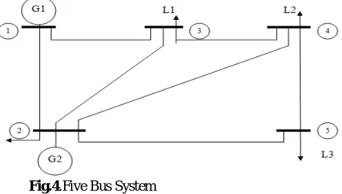
With bus1 as Slack, use Gauss-Seidel iterative method to obtain a load flow solution for the following figure 4 using YBUS with acceleration factors of 1.4 and 1.4 and tolerances of 0.0001 and 0.0001 per unit for real and imaginary
components of voltage.
Fig.4.Five Bus System
Bus code (p-q)
Impedance (Zpq)
Line charging admittance y’pq / 2
1-2 0.02+j0.06 0.0+j0.030 1-3 0.08+j0.24 0.0+j0.025 2-3 0.06+j0.18 0.0+j0.020 2-4 0.06+j0.18 0.0+j0.020 2-5 0.04+j0.12 0.0+j0.015 3-4 0.01+j0.03 0.0+j0.010 4-5 0.08+j0.24 0.0+j0.025
Table: 2 Bus Code ‘p’ Assumed bus voltages
Generation Load
Mega watts Mega vars Mega watts Mega Vars
1 1.06+j0.0 0 0 0 0 2 1.0+j0.0 40 30 20 10 3 1.0+j0.0 0 0 45 15 4 1.0+j0.0 0 0 40 5 5 1.0+j0.0 0 0 60 10
Solution: Step: 1
Calculate the Admittance matrix from the given Impedance and Line charging admittances values. Where the diagonal values are calculated as below.
Y11= y12+y13+y1,
Y22=y21+y23+y24+y25+y2,
Y33=y31+y32+y34+y3,
Y44=y42+y43+y45+y4,
Y55=y52+y54+y5
And the off diagonal elements as shown
Y12 =Y21= -1/z12, Y13=Y31= -1/z13, Y14 =Y41= -1/z14, Y15 =Y51= -1/z15,
Y23=Y32= -1/z23, Y24 =Y42= -1/z24, Y25 =Y52= -1/z25,
Y34 =Y43= -1/z34, Y35 =Y53= -1/z35,Y45= -1/z45 =Y54.
The obtained admittance matrix is as shown below. Ybus=
6.25-j18.695 -5.0+j15.0 -1.25+j3.75 0 0 -5.0+j15.0 10.8334-j32.415 -1.667+j5.0 -1.667+j5.0 -2.5+j7.5 -1.25+j3.75 -1.667+j5.0 12.91667-j38.695 -10.0+j30.0 0
0 -1.667+j5.0 -10.0+j30.0 12.91667-j38.695 -1.25+j3.75 0 -2.5+j7.5 0 -1.25+j3.75 3.76-j11.21
Table: 3 YBUS matrix.
Step: 2 Solving these equations for Gauss-Seidel iterative solution using bus numbers we get bus voltage values. E1=1.06+j0.0,
E2 k+1 = (P2-jQ2) L2/ (E2k)*-YL21E1-YL23E3k-YL24E4k-YL25E5k,
E3 k+1 = (P3-jQ3) L3/ (E3k)*-YL31E1-YL32E2k+1-YL34E4k,
E4 k+1 = (P4-jQ4) L4/ (E4k)*-YL42E2K+1-YL43E3k+1-YL45E5k,
Table: 4 Solved Bus Voltages for the given five bus system.
Step: 3
An acceleration factor ’α’ can be used for faster convergence. As acceleration factor is specified then modified (k+1) th iteration value of bus ‘P’ is done using
Epacck+1 = Epk + α (Epk+1 - Epk) and then assume
Epk+1 = Epacck+1
Step: 4
Calculate the change in bus ‘P’ voltage using the relation
ΔEpk+1 = Epk+1 - Epk.
Then the obtained changes in Bus voltages are as shown.
k
Change in Bus Voltages
Bus 2 Bus 3 Bus 4 Bus 5 0 0.0+j0.0 0.0+j0.0 0.0+j0.0 0.0+j0.0 1 0.05253+j0.00406 0.00966-j0.01289 0.01579-j0.02635 0.02727-j0.07374 2 -0.00724-j0.03421 0.01188-j0.02938 0.00872-j0.03718 -0.07102-j0.01558 3 0.00204-j0.00603 0.00483-j0.02926 -0.00057-j0.01973 0.00687-j0.00894 4 0.00232-j0.01112 -0.00242-j0.01136 -0.00126-j0.00753 -0.00137-j0.00961 5 -0.00215-j0.00286 -0.00095-j0.00404 -0.00120-j0.00314 -0.00260+j0.00005 6 -0.00041-j0.00041 -0.00105-j0.00184 -0.00112-j0.00080 0.00001-j0.00091 7 -0.00030-j0.00070 -0.00089-j0.00024 -0.00059-j0.00020 -0.00060-j0.00035 8 -0.00039+j0.00007 -0.00036-j0.00012 -0.00032-j0.00008 -0.00032+j0.00015
9 -0.00009-j0.00003 -0.00022-j0.00005 -0.00018-j0.00001 -0.00005-j0.00011 1 -0.00007-j0.00003 -0.00012+j0.00001 -0.00007-j0.00002 -0.00008+j0.00000
Table: 5 Shows the changes in bus voltages for 10 iterations.
Step: 5
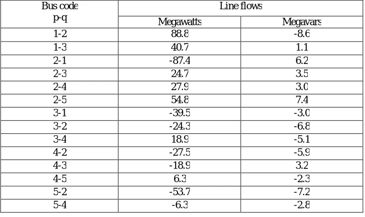
Line flows are calculated with final bus voltages and given line admittances and line charging using the relation,
Ppq – jQpq = Ep*(Ep – Eq)ypq + Ep*Ep y’pq / 2 .
‘k’ Bus Voltages
Bus code p-q
Line flows
Megawatts Megavars
1-2 88.8 -8.6
1-3 40.7 1.1
2-1 -87.4 6.2
2-3 24.7 3.5
2-4 27.9 3.0
2-5 54.8 7.4
3-1 -39.5 -3.0
3-2 -24.3 -6.8
3-4 18.9 -5.1
4-2 -27.5 -5.9
4-3 -18.9 3.2
4-5 6.3 -2.3
5-2 -53.7 -7.2
5-4 -6.3 -2.8
Table: 6 Active and Reactive power flows in the five bus system
The slack bus power can be determined by summing the flows on the lines terminating at Slack Bus. The real slack bus power is 129.5 MW and the Reactive power is – 7.5 MVAR. (ref.no.14)
V. RESULT AND DISCUSSION A: SIMULINK MODEL OF A FIVE BUS SYSTEM
To develop a Simulink model for the above represented data, the values that are required can be considered from the calculated values shown below. These include the actual values of resistance, inductance and capacitance which are obtained from give per unit values of impedance and admittance.
Bus (p-q) R(Ω/km) L(H/km) C(F/km) 1-2 0.0726 6.936 * 10-4 5.25 * 10-5 1-3 0.2904 2.77 * 10-3 4.378 * 10-5 2-3 0.2178 2.08 * 10-3 3.503 * 10-5 2-4 0.2178 2.08 * 10-3 3.503 * 10-5 2-5 0.1452 1.38 * 10-3 2.627 * 10-5 3-4 0.0363 3.468 * 10-4 1.751 * 10-5 4-5 0.2904 2.77 * 10-3 4.378 * 10-5
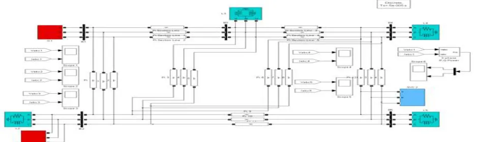
Here the below model represents a five bus system constructed using the sim power systems software. The supply, loads, active and reactive power are considered from the problem.
Fig.5. Five bus system constructed using the sim power systems
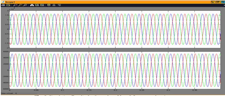
These are the waveforms obtained for voltage and current across the first bus after simulating the above circuit of five bus system and are represented by Vabc1 & Iabc1
Fig. 6.Simulation Results for three phase Vabc1 & Iabc1 across bus 1
B: SIMULINK MODEL OF A FIVE BUS SYSTEM WITH SVC
Here this model represents a five bus system connected with SVC across bus 5 and is constructed using the sim power systems software.
Fig. 8.Simulation Results for three phase Vabc1 & Iabc1 across bus 1
Even though the primary purpose of shunt FACTS devices is to support bus voltage by injecting or absorbing reactive power. They are also capable of improving the transient stability by increasing or decreasing the power transfer capability when the machine angle increases or decreases which is achieved by operating the shunt FACTS devices in capacitive or inductive mode. The proof of maximum increase in power transfer capability is based on the simplified model of the line neglecting line resistance and capacitance. However, for long transmission lines, when the actual model of the line is considered, the results may deviate significantly from those found for the simplified model.
Here at first a five bus system was built by considering the values of the considered problem using MATLAB with given different loads across different buses and then after the same system is shunt connected with SVC and the difference in reactive power was observed before and after.
A simulation result shows that the appropriate location of the SVC provides to control the system voltage at the desired level and compensation of reactive power by using minimum number of SVCs. Here the voltages are maintained at constant levels across the buses.
Therefore it is concluded that the Reactive power is compensated, and also at the same time active power is also improved by the connection of the shunt device called as static var compensator.
REFERENCES
[1] Hingorani, N.G., “High Power Electronics and Flexible AC Transmission System”, Joint APC/IEEE Luncheon Speech, April 19, 1988 [2] Hingorani, N.G., “Flexible AC Transmission systems”-Overview, paper presented IEEE PES1990, February 1990.
[3] Chamia, M., “Power Flow Control in Highly Integrated Transmission Network”, November 1990.
[4] Hingorani, N.G., “FACTS-Flexible AC Transmission systems”, IEE Publication No.345, pp. 1-7, September 1991. [5] Deuse, J., Stubbe, M., Meyer, B., and Panciatici, P., “Modeling of FACTS for Power System Analysis”, May 1995.
[6] Casazza, J.A., and Lekang, D.J., “New FACTS Technology: Its potential impact on Transmission System Utilization”, November 1990. [7] U. Eminoglu, T. Yalcinoz, S. Herdem., “Location Of Facts Devices On Power System For Voltage Control”, 2000.
[8] Hingorani, N.G., “A Text book based on Flexible AC Transmission systems”, October 1998