An Evolutionary approach to microstructure optimisation of stereolithographic models.

An Evolutionary approach to microstructure optimisation of

stereolithographic models.

Siavash Haroun Mahdavi

University College London Gower St. London WC1E 6BT, UK

[email protected]

Sean Hanna

Bartlett School of Architecture University College London Gower St. London WC1E 6BT, UK

[email protected]

Abstract- The aim of this work is to utilize an evolutationary algorithm to evolve the microstructure of an object created by a stereolithography machine . This should be optimised to be able to withstand loads applied to it while at the same time minimizing its overall weight. A two part algorithm is proposed which evolves the topology of the structure with a genetic algorithm, while calculating the details of the shape with a separate, deterministic, iterative process derived from standard principles of structural engineering. The division of the method into two separate processes allows both flexibility to changed design parameters without the need for re-evolution, and scalability of the microstructure to manufacture objects of increasing size. The results show that a structure was evolved that was both light and stable. The overall shape of the evolved lattice resembled a honeycomb structure that also satisfied the restrictions imposed by the stereolithography machine.

1 Introduction

In his influential 1917 treatise On Growth and Form, D’Arcy Thompson describes the processes determining the shape of living organisms as consisting only partly of Darwinian evolution and partly of the external forces imposed on the organism as it grows in its environment. In the case of bone, for instance, he states:

‘Here, for once, it is safe to say that ‘heredity’ need not and cannot be invoked to account for the configuration and arrangement of the trebeculae: for we can see them at any time of life in the making under the direct action and control of the forces to which the system is exposed.’

(Thomson 1917)

While initially intended as an explanation of biology, his work has had a great following among engineers, and it is in the tradition of his proposal that we propose an algorithmic method of deriving an object’s internal structure based partly on evolution, and partly on deterministic structural engineering principles. This structure is analogous to the fibrous interior of bone, both lightweight and strong, to be manufactured by stereolithography, a computer controlled manufacturing process which uses a laser to set a form in a tank of resin. A series of linear structural members ac ting in either

tension or compression traverse the volume of the object to be made and meet at node points, much like a 3D space frame, only rather than consisting of identical members at fixed angles from one another, their position and orientation are de pendent on the forces that the object is to carry.

Stereolithography builds the entire structure as a unit, so complexity costs nothing. With a resolution of 0.05mm, the process can currently build the structural members under a millimetre in length resulting in a material similar in texture to sponge. This material could be formed to any shape required, and be organized at the smallest scale to carry external forces most efficiently.

In a very basic example of an evenly loaded rectangular beam for instance, points above the central axis are in horizontal compression, and points below are in horizontal tension, and these forces increase vertically from this axis, and decrease horizontally from the centre of the beam, see Fig.1. Rather than adding and removing large areas of material from the beam’s cross section as in the case of a typical ‘I’ cross section, the small scale structure at each point of the beam can be optimised for its structural capacity and least weight see Fig.2.

Fig.1 A simply loaded beam.

Typically structural optimisation methods seek to minimize the weight of a structure capable of withstanding a given set of forces. The work presented here is the first step in forming more complex structures than the simple beam; at this stage we present a method which is scalable in terms of both size and complexity, and produces a generic internal structure which is not under specific loading conditions. External forces are assumed to be in equilibrium and therefore the structure has a regularity at the intermediate scale, but the method is set out for increased complexity in the future.

2 Background

2.1 Structural Optimisation: Previous Work

Several techniques have been devised for generating the topology of continuous solids analysed by the Finite Element Method (FEM). Both GA and non-random iterative methods have been used. Marc Schoenhauer reviews a number of GA methods for generating topology in 2D or 3D space to optimise structural problems involving continuous shapes. The genetic representation in these cases can determine a configuration of holes and solid using Voronoï diagrams or a list of hole shapes (Schoenhauer 1996). Yu-Ming Chen uses a non-random iterative process of shifting node points in the FEM representation toward high stress zones to examine similar problems (Chen 2002). These methods can determine the number and position of holes in a cantilevered plate, for instance, but do not deal with truss-like structures.

The majority of research into the optimisation of discrete element structures (trusses, space-frames) has been in the refining of the shape or member sizes, rather than the topology (in terms of members connecting the node points of the structure). Adeli and Cheng use a GA to optimise the weight of space trusses by determining the width of each member in a given structure. The shape and load points are fixed in advanced, and the cross sectional areas of groups of members are encoded in the genome, then selected to minimize the total weight (Adeli and Cheng 1993). Yang Jia Ping has developed a GA which determines both shape and topology, however the algorithm must begin with an acceptable unoptimised solution and refine the topology by removing connections (Ping 1996).

2.2 Stereolithography: Previous Work

Stereolithography and other rapid prototyping techniques are now beginning to be investigated as an alternative method of construction for objects of high complexity, particularly with intricate internal structures. This has not yet become commercially viable for mass production, but several researchers are preparing for the increasing accuracy and decreasing cost of the technology in the future. Molecular Geodesisics, Inc. is investigating structures based on a regular tensegrity space frame which would, at a microscopic size, be useful as biological or industrial filters (Molecular Geodesics 1999).

2.3 Stereolithography: The Process

Stereolithography is a method of creating solid 3D models of CAD drawings, see (Brain 2002) for a fuller explanation. It is one of the many types of machines collectively called ‘rapid prototyping machines’. As the name suggests, the ir primary usage is with the rapid building of prototypes for testing by engineers and designers. However as the technology has been dramatically improving over the past several years, it has become evident that this process can be used for more than building prototypes and can be itself a method for constructing parts.

The stereolithography machine consists of a tank filled with liquid photopolymer which is sensitive to ultraviolet light. An ultraviolet laser ‘paints’ one of the layers, exposing the liquid in the tank and hardening it, a platform then drops down into the tank a fraction of a millimetre and the laser paints the next layer. This process repeats until the model is complete.

Once completed, the object is rinsed with a solvent and then baked in an ultraviolet oven that thoroughly cures the plastic.

3 Method

3.1 Overview

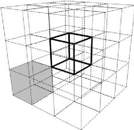
Fig. 3. An array of 26 outer cubes surrounding the central cube.

Two separate processes are used to determine the structure: the connections between nodes evolved by a genetic algorithm (GA) and their positions by a deterministic analysis of the forces. Given n points in space, a graph of connections (the ‘connection graph’) can be formed between them that does not vary topologically as the locations of any of the points change. The number of possible graphs is ‘n factorial’, and it is this connection graph between the nodes that the GA evolves. This process takes some time and by its nature involves randomness. The actual position of the nodes however, is determined by a separate, iterative process of moving points in space to achieve structural equilibrium. This standard analysis of structural equations is deterministic and efficient. The placement of the node points in 3d space varies from point to point, but their connections to one another does not. This accomplishes two things that we find necessary for scalability. First, it avoids breaks in the continuity of the structure by allowing a difference between one unit cube of structure and the next which can be scaled to arbitrary units of precision. These break points would literally be break points if the connection graph were to change, as adjacent units of incompatible structures would be zones of weakness in the overall object. Second, it allows one single graph of connections to be evolved which can be applicable to all points. This allows an object of any size and any number of units to be evolved once, rather than running the GA many times to

generate structures for large objects or complex load conditions.

Analysis of an overall complex shape or complex loading is a standard procedure usually performed by the finite element method (FEM) and by many existing software applications, as such it is not considered in this paper. Instead, the work presented here is the creation of a structure at the simple end of this range, designed to test the method. Evolution is performed to optimise the connection graph under a range of differing tensile conditions but the overall object is not subjected to complex loads at varying points, and as such, the final position of nodes in each unit cube does not vary.

3.2 Geometrical Representation

Associated with each unit cube are n points that define the nodes at which two or more linear structural members meet. The structural members forming connections between these points are determined by the connection graph evolved by the GA and their size and the location of node points determined by the iterative process described below. Each node point may be connected to any number of other points in either its own unit or any adjacent unit to form a basic structural unit of the design, repeated in each unit cube of the structure. Although the unit cube defines a volume of space, the node points are not constrained by it and are free to extend this structural unit beyond any of the boundaries, thereby overlapping the adjacent structural unit.

Each point may be connected to any of the (n – 1) points in its own unit, or any of the 26 (including corner adjacencies) adjacent cubes, for a total of (27n –1) possible connections to each node point, see Fig. 3.

4 Iterative Structural Analysis

4.1 Methods of Analysis

Standard vector methods were used in the analysis of the structures. Given a tensile or compressive force F acting in the direction of the structural element this can be decomposed into its (x,y,z) components along each of our axes. For each node point to be in a state of equilibrium, all of its connecting members are considered using the element analysis equations, such that:

S

S

S

The structure is analysed as a pin jointed system rather than a frame in bending, so no moments need be considered in the equations.

4.2 Iterative Determination of Node Positions

While the GA generates the pattern of connections, the actual position of node points in space is determined by a deterministic process involving no randomness. These are based purely on the connection graph and the given direction and size of forces acting on each point in the structure. Given a connection graph indicating which nodes are to be connected to one another, the location of each node in space is determined by an iterative process which moves each node from an initial start point in the direction required to bring the forces in each connected member into equilibrium. To begin the process, all nodes are placed at the origin (0,0,0) point in 3d space. For each iteration the list of node points is traversed, and the (x,y,z) coordinates of each point updated to the weighted average of the coordinates of all points to which it is connected. Thus the node points are pulled from the centre of the unit cube in the directions of the adjacent cubes to which they are connected. The process is stopped when the maximum movement of any point is within a given tolerance (0.1 units) or after a set number (500) of iterations.

All points are moved at each iteration, therefore the structure tends to oscillate around a solution. Often the ideal points are converged upon quite quickly but sometimes the process continues for more than the maximum number of allowed iterations. If this occurs the given points are considered to have been oscillating around a state of equilibrium, and have therefore not yet found a solution. Thus the points are less fit and the solution is penalized in the fitness function of the GA. Also, because there are no fixed points in the structure, the entire set of points could move in space as equilibrium is established between the members. At each iteration therefore, the mean coordinates of the entire set of points is reset to the origin.

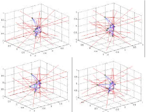
As mentioned above, the evolved connection graph is meant to be viable (with some translation of node positions) under a range of tensile or compressive forces in any direction. Weighting the above calculation in the direction of the forces to be applied simulates different loading conditions for each unit cube. The stereolithography resin is able to act in both tension and compression so one set of tensile calculations was used for both. To weight the calculation of the node position, applied forces are broken into their respective (x,y,z) component vectors as are each of the members in the calculation, and the node point with its connecting members treated as an isolated structural unit under those forces, to be solved by the element analysis equations. The different component vectors of the applied tensions are divided between the unit vectors of the members, and the resulting tension solved by the element analysis equations used to weight the averaging calculation. Thus under different loading conditions the shape of the structure is seen to shift to accommodate the change in forces, see Fig. 4.

Fig. 4. A unit cube that has been orientated to remain in equilibrium when exposed to forces coming from different directions. (Equal tension in all axes, then 5:1 in the x, y and z axes respectively.)

The efficiency of the calculation is improved by taking advantage of the fact that there is a greater difference in the position of the points found under each load condition and their starting point at the origin than between either of the different solutions found. The point locations are first found for an equally tensioned condition, that is a tension of one unit along each axis, and this result is then used as the starting position for each of the other conditions. A tension of five units was used for each of the (x,y,z) axes in sequence.

4.3 Analysis of the Solution by DSM

The resulting solution is a list of fixed points in space connected by members of known length and orientation is then evaluated for deflection using the direct stiffness method. The set of all nodes in the unit, with their internal connections and those to adjacent unit cubes, are considered as an isolated structure placed under the applied external forces. The deflection of each member is calculated, and these used in the fitness function to assess the solution.

5 Material considerations

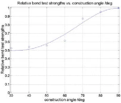
In construction, the structure is formed in a liquid stereolithography resin as a series of horizontal layers. This results in an inherent horizontal ‘grain’ in every part of the model and an inability to construct the underside of any portion at an angle of less than 30º from horizontal. Members constructed at differing angles to this ‘grain’ therefore have differing strengths and their calculated deflections were modified accordingly in assessing the fitness of the solution.

this data with all angles below 30º at a strength of zero, see Fig. 5. Then, in determining deflection for the fitness function, the calculated deflection of all members was divided by the value of this function. The method for calculating the strength of the struts was one used for testing the strength of fibres. This method, bend strength testing, is a standard method of evaluating the strength of a fibre or a thin rod that cannot be compressed without it bending. An equation then relates this bend strength to the compressive strength of the strut.

Fig. 5. Plot of the angle vs. relative strength.

The stereolithography machine used has the ability to manufacture geometry to a resolution of 0.05mm. However because the liquid resin has to drain from anything built in the machine, and the designed structure is full of holes, an experiment was done to investigate the minimum size hole from which the resin could drain. A plate was constructed with holes ranging in radius from 5mm to 0.05mm. It was observed that the smallest hole from which resin could drain was 0.6mm. This was taken into consideration when deciding on a scale to construct the structure.

6 The Genetic Algorithm

6.1 Chromosome Structure

The genetic algorithm is used to evolve the connection graphs, which describe the connections between the nodes. The structure of the chromosome is a series of upper triangular matrices (UTM) that describe the connections of these nodes to one another. The first UTM describes the internal connections of the n nodes within the cube. The other 26 UTMs describe connections between the nodes within the original centre cube and the copies of themselves in the surrounding cubes. Below is an example of the 27 UTMs when just four nodes are used, see Fig. 6.

Fig 6. An example of the 27 UTMs using 4 nodes.

If any point row contains entirely zeros this indicates a lack of connections and the point is effectively eliminated from the structure. The chromosome is constructed to allow this to occur as an implicit method of simplifying the overall structure. If such a simplification occurs under crossover and mutation and is found to increase the fitness by reducing weight and still maintaining a stable structure this will be likely to influence future generations, gradually reducing the effective number of points over time.

6.2 Initial Population

For the initial population, each bit is created randomly. The probability of having a 1 in the first UTM (connection between two internal nodes) is 0.5. By intuition, the probability of having a 1 in any of the other UTMs is set to around 0.03 (connection between internal nodes and the copies of themselves in the surrounding cubes). This low value was selected as an equal number of each bit would result in far too high a number of connections, and as evolution would bring this number down over time. Thus a head start was given. This assumption was verified as the number of cross cube connections decreased from 0.03 to 0.0016 during evolution in the longest run of the algorithm, presented in Section 7.

6.3 Crossover

The point numbers have no effect on the topology of the connection graph, so the numbering of the points is arbitrary. The crossover function is therefore not performed by taking a whole length along the chromosome, instead x randomly chosen points from all the 27 UTMs are taken from each parent and the two corresponding values are swapped. The final crossover rate used was 30%.

6.4 Mutation

The mutation mechanism is separated into two types: one for the central cube and another for all of the other surrounding cubes. For the central cube, a number of mutation points are chosen, depending on the mutation rate, and these bits are then flipped (0 replaced with 1 or vice versa).

As each mutation is intended to forge or break connections with similar probability, the sparseness of the connection graph for the surrounding cubes requires the mechanism for the rest of the cubes to be a little different. Because of the very large number of 0s in these outer cubes, if a standard mutation was carried out on random bits, then the number of external connections would dramatically increase in the following generations. To overcome this, the program decides on whether to flip a 0

1 2 3 4 1a 2a 3a 4a 1b 2b 3b 4b 1z 2z 3z 4z 1 0 1 1 0 0 0 1 1 0 0 0 0 ... 0 0 0 0 2 0 0 1 0 0 0 0 1 0 ... 0 0 1

3 0 1 0 0 0 0 ... 0 0

or 1 with a probability of 0.5. If a 0 is chosen, one of the 0s in the outer UTM is found randomly and flipped. If a 1 is chosen, one of the 1s in the outer UTM is found randomly and flipped. This has the effect of mutation and can over time vary the proportion of 0s and 1s.

6.5 Fitness Function

The factors taken into consideration when determining the fitness of each individual in the population are as follows:

• The number of angles below 30o • The overall weight of the individual • The maximum deflection within the system • Whether the iterative node placement had found a

solution that settled down

The effect of each one of these factors was weighted as follows .

The values of A and C have to simply be high enough to ensure that individuals with angles below 30o (a material constraint) and those that are not in equilibrium have a significantly lower fitness.

The values of W and D were chosen so that the weight of the structure and its strength have a roughly equal importance. These four variables were then put into the following equation for each test under a different stress condition (T):

T = 1 . (1 + A×lowAngles + W×weight + D×maxDeflection + C×count)

The fitness of each individual was then the sum of the Ts for each of the four test.

6.6 Selection

The individuals in the population were selected using roulette wheel selection. The genetic algorithm was elitist in that the top two individuals of each generation were placed directly into the next generation. This meant that the fitness of the best member of the population at each generation never decreased.

7 Results

The population size was set at 50 and the program was run for 10,000 generations. The time taken for e ach individual was about half a second (all four test conditions) making the total time taken to run the whole experiment around three days.

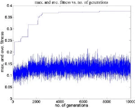
The following plot displays the fitnesses over time for the longest of several test runs of the combined algorithm. This resulted in the structure with the highest fitness found. The plot shows the maximum and average fitness

of the individuals at each generation, see Fig. 7. These values start, in the first generation, at a maximum value of 0.0575 and an average value of 0.0322. By the end of the final generation, these values increase to 0.3766 and 0.1580 respectively.

Fig. 7. A plot of the maximum and average fitness at each generation.

8 Analysis

In the course of several test runs, the following were observed:

• The number of connections to adjacent cubes always decreased.

• The number of internal connections always decreased.

• The angles of the members always increased beyond 30° with a preference for steeper angles. • Point reduction over time was observed.

The diagram of a single unit of the best individual found from the plot shown in Fig. 7 is depicted below, see Fig. 8. It is worth examining this structure in more detail. This solution is noticeably simpler than an average solution found in the early stages of evolution, see Fig. 9. The number of outer cube connections has also dropped considerably to only three.

Fig. 8. A unit cube of the best individual evolved.

Fig. 9. A unit cube of an average individual evolved.

As mentioned in Section 6.1, the simplification of structure by point elimination is possible over time. This has occurred here. Of the twelve initial points in the connection graph, two have been effectively eliminated from the solution by removal of all their connections to other points.

As can be observed in the unit cube diagram, the solution is not an obvious one. However once the individual unit is arrayed, one can see that a very interesting solution has been evolved. The shape of the repeating pattern very much resembles that of a honeycomb structure. Seen from above, the structural members are aligned to the edges of a tiled pattern of almost regular hexagons with approximately equal angles. When viewed from the side however, near vertical elements predominate due to the material constraints mentioned previously: because the hardened photopolymer has a greater structural strength at steeper angles, the structure appears elongated in this direction. Also, no members at an angle of less than 30o are found. Both the satisfaction of these constraints, and the shape of the honeycomb structure can be seen in Fig. 10 below.

Fig. 10. The top and side views of the final structure evolved.

The module can be repeated as a unit cube to manufacture the final object of any size. The resulting structure is self-supporting and optimized for the material properties of the liquid photopolymer, the stereolithography process and an identical stress condition throughout, see Fig. 11.

Fig. 11. A 10 x 5 x 5 example of the evolved structure.

9 Conclusion

The aims were to generate a repeatable structure which minimised weight and maximised strength, while considering the specific properties of the material in which it is built. This was to have the ability to transform continuously to accommodate the range of forces which may be present in the object without the necessity of re-evolving the structure.

The method of representing the connection graph in a genome comprised of UTMs is a straightforward method which yields good results under the mutation and crossover operators. The number and size of structural members was seen to decrease over the course of the run while maintaining a stable and viable structure within the constraints provided.

solution generated for the particular properties of the material and a given range of forces can therefore be quickly modified to the redesign of the object or a new stress distribution without rerunning the algorithm.

10 Future Work

As previously discussed, throughout this work, the values of force, displacement, weight etc. were not selected for a specific problem, but were chosen in arbitrary units to test the algorithm. Of primary importance was that the final evolved product had reduced its overall weight to strength ratio. Future work would involve simulating a specific task with very specific weight and strength requirements, and subjecting the evolved structures to rigorous laboratory testing.

The algorithm presented evolves a generic unit of connections which can be made to accommodate the specific forces presented in given real world problems . Future work would involve constructing objects which, while under these specific loading conditions, have a variety of differing node placements in each unit cube. These nodes will vary continuously throughout the object to accommodate the change in direction of the applied forces on that point, and member widths will vary to accommodate changes in magnitude. These local effects are seen as the tools for a larger scale optimisation as described in the example of the ‘I’ cross section beam in Fig. 2. As such these tools will be applied to problems of greater complexity.

Acknowledgments

We would like to thank Thomas Modeen for his continuing investigation into novel applications for rapid prototyping techniques, and Chris Williams for his knowledgeable advice and inspiring structural engineering methods.

References

Adeli, Hojjat and Cheng, Nai-Tsang. (1993) “Integrated Genetic Algorithm for Optimisation of Space Structures,” Journal of Aerospace Engineering, Vol. 6, No. 4.

Brain, Marshall.(2002) “How Stereolithography Works,” www.howstuffworks.com/stereolith.htm.

Chen, Yu-Ming, (2002) “Nodal Based Evolutionary Structural Optimisation Methods,” PhD Thesis, University of Southhampton.

McGuire, W., Gallagher, R. H. and Ziemian, R. D. (2000) “Matrix Structural Analysis,” 2nd edition.

Molecular Geodesics, Inc. (1999) “Rapid prototyping helps duplicate the structure of life,” April 99 Rapid Prototyping Report.

Ping, Yang Jia. (1996) “Development of Genetic Algorithm Based Approach for Structural Optimisation,” PhD. Thesis, Nanyang Technological University.

Schoenhauer, Marc. (1996) “Shape Representations and Evolution Schemes,” Proceedings of the 5th Annual Conference on Evolutionary Programming.