Pair Programming and the Factors Affecting Brooks' Law

(1)

Abstract

SHUKLA, ANUJA. Pair programming and the factors affecting Brooks’ Law.

(Under the direction of Dr. Laurie Ann Williams).

Frederick Brooks states in his book The Mythical Man-Month, “Adding manpower to a late software project makes it later.” Brooks explains that often software development managers react to schedule problems by adding more manpower to the project. However, the new team members take some time initially to be

trained and assimilated into the project. Assimilation time is the time the new team member takes to understand project specific details. Also, if the subprojects assigned to each engineer are interrelated, intercommunication requirements rise since each part of the task must be separately coordinated with each other part. Thus, Brooks contends that when manpower is added to a late project the overall productivity goes down, delaying the project even further.

This research investigates the effects of pair programming on the training, assimilation and intercommunication, as mentioned in Brooks’ Law. Pair

(2)

pair rotation practices. Through surveys and mathematically modeling, we found the following:

1. Pair programming reduces intercommunication time within a team.

2. Pair programming reduces mentoring time when new members are added to a team.

3. Pair programming reduces assimilation time when new members are added to a team.

(3)

PAIR PROGRAMMING AND THE FACTORS AFFECTING

BROOKS’ LAW

by

Anuja Shukla

A thesis submitted to the Graduate Faculty of North Carolina State University

in partial fulfillment of the requirements for the Degree of Master of Computer Science

Department of Computer Science

Raleigh

May 2002

Approved By:

_________________________________________ Dr. Laurie Williams

Chair of Advisory Committee

(4)

Biography

(5)

Acknowledgements

This work was possible only with the continuous guidance, support, coaching, and mentoring of my advisor Dr. Laurie Williams. She not only guided me through this process but also encouraged me to participate in various

conferences and helped me broaden my perspective. I would like to extend my appreciation to the committee members, Dr. Annie Antón and Dr. Thomas Honeycutt.

(6)

1. Introduction

1.1 Research Motivation

Software projects often run behind schedule and over budget. A Standish Group [1] study shows a staggering 31.1% of projects are canceled before they are ever completed. Further results indicate 52.7% of projects cost 189% of their original estimates. Only 16.2% of software projects are completed on time and on budget. And, even when these projects are completed, many reflect no more than a mere shadow of their original specification requirements. Projects completed by the largest American companies have only approximately 42% of the originally proposed features and functions [1].

Furthermore, late delivery of software prevents the use of the software and opportunity to make profits from the product. These lost opportunity costs are not measurable, but could easily be in the trillions of dollars. The Standish Group also estimated that in 1995 American companies and government agencies spent $81 billion for canceled software projects. These same organizations paid an additional $59 billion for software projects that were completed, but exceeded their original time estimates [1].

While software technologies, processes, and methods have advanced rapidly, software engineering remains a people-intensive process. As a result, there is much emphasis on techniques for managing people, technology,

(11)

environment to facilitate interactions amongst colleagues and peers; these organizations promote teamwork, training, collaboration etc.

Teams often encourage knowledge sharing between members who have diverse intellectual and occupational backgrounds. Research studies [2] indicate that team collaboration is known to have a positive effect on the team morale and productivity, which improves the workplace environment. By applying knowledge management techniques, such as knowledge discovery, knowledge capture, and information retrieval and extraction, companies and organizations can improve their ability to create, acquire, disseminate, and retain knowledge; thereby enabling them to make effective decisions, control complexity, and improve productivity.[2] By disseminating individual’s knowledge throughout an

organization, knowledge loss due to employee turnover can be minimized. With the realization of the value of knowledge assets, companies and organizations increasingly seek to implement knowledge management techniques to increase their effectiveness [2]. Knowledge management techniques can be useful in software project management to facilitate on time product delivery.

(12)

three important factors that explain why more man-power does not necessarily mean more work is effectively accomplished:

1. Increased training costs. This cost varies linearly with the number of people.

2. Increased assimilation time. This cost varies linearly with the number of people.

3. Increased communication overhead. This increases non-linearly as more people are added to a team.

When new people are given tasks to be performed, they need training on the technology, the goals of the effort, and the overall strategy. They cannot immediately undertake tasks and contribute to the project. They require some time in order to be assimilated. As a result, new team members start off with a lower productivity, which gradually increases with training. Also, more members on a team imply increased intercommunication overhead when tasks are

interrelated; team members must speak with all other team members. When more people are added to a team, it is observed that amount of code generated per programmer decreases [4].

(13)

productivity creates delays, which motivates additional hiring, which leads to severe losses in productivity, further delays, more hiring and so on [5] .

This research study investigates the effects of pair programming on the factors affecting Brooks’ Law: training, assimilation, and intercommunication time. With pair programming, two programmers working side-by-side at one computer, collaborating on the same design, algorithm, code, or test. One programmer is the driver, controlling the input device (keyboard and mouse) to produce the design or code. The other programmer is the navigator,

continuously and actively examining the driver’s work. This research investigates the potential of pair programming to alleviate the effects of training, assimilation, and intercommunication costs:

• Training. A person new to a project cannot start contributing immediately

towards the overall productivity. Thus, the time spent on training is

significant and has to be considered in project schedule estimation. New team members are generally trained by a mentor, an experienced peer, who is familiar with all the project details. The mentor introduces the new member to project details as well as non-technical matters of how to be effective and successful in the organization. While mentoring, the

(14)

details to the new team member. With pair programming, the mentoring time is the fraction of the day spent when the experienced person pairs with a new person vs. when the mentor pairs with another experienced person.

• Assimilation time. This is the time required for a new project staff

member (who already possesses the necessary knowledge and skills) to become an effective, contributing team member. This includes helping a new recruit understand project-specific facts, such as facility layout, policies, procedures, development domain, and development and the test environment.

• Intercommunication time. Intercommunication time includesverbal

communication, documentation, and any additional work required to communicate, formally or informally, among the team members.

Introducing informal means of communication within a team is a good way to reduce communication overhead. Rather than involving all team

(15)

1.2 The Research Approach

The objective of this research is to analyze the effects of pair programming on the factors affecting Brooks’ Law, to see if pair programming has a positive effect on, mentoring, assimilation and communication overhead. Specifically, we investigate the following hypotheses:

• Pair programming reduces intercommunication time within a team.

• Pair programming reduces mentoring time when new members are added

to a team.

• Pair programming reduces assimilation time when new members are

added to a team.

• Manpower can be added to a late software project provided the additional

useful effort delivered to the project is adequate to achieve the desired schedule. Pair programming can make this more achievable.

The impact of pair programming on intercommunication is examined by charting the number of communication paths on a team and via mathematical modeling. Mentoring and assimilation factors were examined based on survey results and a mathematical model developed by Stutzke [19].

1.3 Summary of Remaining Chapters

(16)

Chapter 3. BROOKS’ LAW contains an explanation of the law and the effect of factors such as assimilation, communication overhead and training of newly hired work force.

In the past two decades, there have been several analyses of Brooks’ Law [3]. Chapter 4. STUTZKE’S MATHEMATICAL MODEL presents one such

analysis. The model analyzes the process and costs of assimilating new team members, including the costs associated with the diversion of their mentors from the project task itself.

Chapter 5.SURVEY RESULTS contains an analysis of the data obtained by the surveys with respect to assimilation and mentoring times.

Chapter 6. PAIRING AND INTERCOMMUNICATION. The chapter discusses the effects of pair programming on communication overhead and explains how communication overhead is reduced, as it cuts the necessary communication paths nonlinearly.

(17)

Chapter 8.CONCLUSIONS summarizes the conclusions and contributions of the thesis.

Chapter 9. FUTURE RESEARCH suggests future research in areas of pair programming.

(18)

2. Pair Programming

"There is no "I" in the word team." Anonymous

2.1 Pair Programming

Pair programming is a style of programming in which two programmers work side-by-side at one computer, continuously collaborating on the same design, algorithm, code, or test. One person, called the driver, is responsible for typing at the computer or documenting a design. The other partner, called the navigator, has many jobs: he or she observes the work of the driver, looking for tactical and strategic defects in the work of the driver. Tactical defects are syntax errors, typos, calling the wrong method, etc. Strategic defects are identified when the driver is perceived to be headed down the wrong path (e.g., what they are implementing will not achieve the desired result). The navigator is the strategic, long-range thinker. The navigator must adopt an objective point of view so as to think strategically about the work’s direction. Additionally, the driver and the navigator can brainstorm on-demand at any time [6]. Even when one programmer is significantly more experienced than the other, it is important to take turns driving, lest the observer feels out of the loop or unimportant. The navigator is not a passive observer, instead he/she is always active and engaged [7].

Pair programming has been practiced sporadically for many years [6]. However, pair programming has recently been popularised by Extreme

(19)

XP advocates pair programming with such fervour that even prototyping done solo is scrapped and re-written with a partner. One key element is that while working in pairs a continuous code review is performed, noting that it is amazing how many obvious but unnoticed defects become noticed by another person watching over their shoulder. Results

demonstrate that two programmers work together more than twice as fast and think of more than twice as many solutions to a problem as two working alone, while attaining higher defect prevention and defect removal, leading to a higher quality product [9].

2.1.1 Benefits of Pair Programming

Investigative studies [10] have shown that pair programming has inherent benefits, including:

• Continuous Reviews. Pair programming’s shoulder-to-shoulder

technique serves as a continual design and code review, leading to more efficient defect removal rates as compared to two solo

programmers.

• Problem solving. Experienced pairs refer to the team's ability to

solve "impossible" problems faster.

• Learning. Pair programmers repeatedly cite how much they learn

(20)

• Team Building and Communication. Pair programmers become

more familiar with each other, which serves to improve team communication and effectiveness.

• Knowledge Management. Research shows that pair programming

is an effective Knowledge Management technique [2]. In the course of pair programming, multiple programmers are exposed to each piece of code, reducing the impact of losing staff. When a pair is split, they both take domain and coding knowledge to other programmers that they pair with in the future. The continual interaction between pair programmers provides an environment that promotes knowledge sharing, and collaborative knowledge discovery [2].

• Quality and Productivity. Studies have demonstrated through

anecdotal, qualitative and quantitative evidence that incorporating pair programming into a software development process will help yield software products of better quality in less time with happier, more confident programmers [13]. Developers are less likely to produce defective code, because a teammate is watching them. Developers are less likely to spend time on things other than work; therefore productivity increases [10].

(21)

with only a minimal increase in prerelease programmer hours. [10] Initially, the students took, on average, 60% more programmer hours to complete the assignment when compared to individual programmers. After an initial

adjustment period, the additional time decreased dramatically to a statistically insignificant minimum of 15%. Because the pairs worked in tandem, they were able to complete their assignments 40-50% more quickly [11].

“Two heads are better then one” is an age-old adage. When people need information or are attempting something new, they often intuitively contact peers or colleagues who have the information or who have had a similar experience. In this way, information can be acquired in a short time and valuable insights can be gained. Pairing contributes to knowledge sharing amongst the team members. Research in the area of knowledge management and pair programming by Palmieri [2] demonstrated a statistically significant positive correlation between the amount of pair programming performed and the effectiveness of the

(22)

2.2 Pair Rotation

Pairing with one partner for the entire project duration is beneficial, but may not be optimal. The term pair rotation is used to denote when team members pair with different team members for varying times throughout a

project. The amount of explicit, deliberate communication to coordinate tasks can also be further reduced with pair rotation. Each team member works with other developers and, in the process, explains his work and learns from his or her partner.

The advantages of rotating the programmers are that they learn more about the whole product by pairing with many team members, they team with the person who can help them the most on a particular task, and communication and teamwork increases significantly [6]. Discussions about interfaces are much shorter since programmers are more familiar with each other’s code or they pair with the programmer who code interfaces with their own. Rotating pairs offers knowledge management benefits because there are always at least two

(23)

3. Brooks’ Law

3.1 An Introduction to Brooks' Law

Fredrick Brooks headed the IBM team that created the first large-scale computer operating system in the early 1960s. Brooks’ Law, articulated in his classic The Mythical Man-Month, has been widely cited for more than 25 years:

“Adding manpower to a late software program makes it later.” [3] He bases his conclusions on the additional linear overhead needed for training and assimilating as well as the nonlinear communication overhead (a function of the square of the number of people) of adding new people to a team [12]. He further explains the various causes for software schedule delays and budget overruns.

• Optimism of programmers. A common reason for overruns is that

programmers are often overly optimistic. They will look at a task and determine the minimum amount of time required to achieve that task. The medium is tractable; the programmers expect few difficulties in implementation. But their ideas themselves are faulty, so they have bugs [13]. Too often, programmers do not anticipate the inevitable unforeseen circumstances and obstacles that cause project slippage. Among the most common are: hardware

(24)

• Confusing effort with progress. The estimating techniques

adopted by project managers are built around cost accounting, and they confuse effort and progress. These techniques imply that more effort leads to increase in progress [13].

• Poor monitoring of schedule progress. Techniques proven and

routine in other engineering disciplines are considered radical innovations in software engineering [3].

• Regenerative schedule cycle. As previously discussed, the first

recourse of managers, when they suspect the schedule is tight, is often to add more staff. Adding people to a software project increases the total effort necessary in three ways: the work and disruption of repartitioning tasks among team members, training the new people, and added intercommunication. They fail to call to mind Brooks’ long-standing advice: “When schedule slippage is recognized, the natural (and traditional) response is to add manpower. Like dousing a fire with gasoline, this makes matters worse, much worse. More fire requires more gasoline, and thus begins a regenerative cycle which ends in disaster [3].” The number of months of a project depends upon its sequential

(25)

Consider a task estimated to be a 12 person-months effort. Three individuals are assigned to the task, thus the task will be completed in four months. There are four measurable milestones (A, B, C, D) which are scheduled to fall at the end of each month [Figure 3.1], taken from [3]

FIGURE 3.1.MEASURABLE MILEPOSTS FOR A 12 MAN-MONTH EFFORT (SOURCE:[3])

Let us suppose the first set of deliverables is not ready until the end of the second milestone. Six person-months of work should have been completed in the first two calendar months, but only three person-month of work was

completed. The project manager considers the following alternatives:

(26)

[3], nine person-months of effort remain and only two months are left to complete the task. The project manager chooses to add two individuals to the existing team of three persons.

FIGURE 3.2.MISESTIMATING IN FIRST PART OF THE TASK (SOURCE [3])

(27)

FIGURE 3.3.MISESTIMATING OF ENTIRE TASK (SOURCE:[3])

Let us consider the regenerative effect for the alternative 1. The two new individuals added to the team, however competent, will require training in the task by one of the three experienced individuals. If this training takes one month, three person-months will have been devoted to work not in the original estimate which did not include this training time. Also, the tasks, originally partitioned among three persons, will now have to be repartitioned amongst five persons. As a result, some work already done will be lost, and the system testing must be lengthened.

(28)

development effort has not progressed. Thus there is no positive effect of adding the two additional resources.

FIGURE 3.4.TRAINING TIME (SOURCE:[3])

We observe from Figure 3.4, at the end of the third month the situation has still not improved. The first milestone has not been reached in spite of the managerial effort i.e. additional hiring and repartitioning of work. Thus, there will be a strong temptation to repeat the cycle of adding yet more manpower.

In alternative 2, the training, repartitioning, and system testing effect will have an even more disastrous effect, leading to a poor quality product.

3.2 Strategies for Software Management

(29)

increasing the size of the team [14]. Each of these strategies will now be examined.

3.2.1 Reduction of Software Size

There is a distinct correlation between software size, as measured in lines of code (LOC) or function points, and development time, effort (e.g.,

man-months, man-years, cost), manpower, productivity, and the number of defects [15]. Software size can be reduced by paring the less essential functions from the software or by deferring the development of functions not needed

immediately [14]. Either of these reduces the scope of the project. In order to salvage a troubled project, reducing the size of the software can lead to a

reduction in development time, effort, the number of defects, and improvement in programmer productivity.

3.2.2 Increasing Project Schedule/Team Size

According to Brooks, more software programs have gone awry for lack of calendar time than for all other causes combined [3]. Why is this cause of

disaster so common? When you set your schedule to the minimum development time, effort is at its maximum to meet deadlines, but the number of defects is also correspondingly high [15].

(30)

the task on the compressed schedule [14] . In addition, the number of defects will drop. It has been found for the average project of 100,000 source lines of code, the large teams (more than 20 people) created over five times as many defects when compared with small teams (fewer than five people) [16] . However, extending the schedule timelines is often not possible once the program is well underway. If your program is in the 12th month of a 12-month schedule, it is just too late to decide you should have planned in terms of a 17-month schedule [14].

Brooks’ well-known observation rings true. The expected advantage from splitting development work among N programmers is O (N) (that is, proportional to N), but the complexity and communications cost associated with coordinating and then merging their work is O(N2_{) (that is, proportional to the square of N)} [17].

Let us further analyze the above statement. A study demonstrated the amount of code generated by a single programmer decreases as more

(31)

increased costs of communication when multiple programmers work on a single project. [4]

Quoting Brooks,

“Intercommunication is worse. If each part of the task must be separately coordinated with each other part, the effort increases as

(where N= number of people in a team).

Three workers require three times as much pair-wise intercommunication as two; four requires six times as much as two...Since software

construction is inherently a systems effort…an exercise in complex

interrelationships…communication effort is great. Adding more men then lengthens, not shortens, the schedule. [3]

3.3 The Dynamics of Brooks’ Law

Hsia, Hsu & Kung [18] support Brooks' Law. They contend that the dynamics of Brooks’ Law starts when the management brings new staff into a project. As a result, there are three effects, as explained below:

• an increase of communication and training overhead;

• an increase of the amount of work repartitioning; and

• an increase of the total manpower available for project

development.

When new staff members are brought in, they require a certain level of training, which will take away part of existing staff member’s productive time.

(32)

Also, an increase in the number of people leads to an increase in

communication. As a result, the total effective project manpower resource also decreases. This results in project progress being delayed even further and leads to another round of people-hiring feedback loop. The increase in the cost of the project is caused by the increased training and communication overhead, which, in effect, decreases the productivity of the average team member and thus increases the project’s person-day requirements.

The second effect of bringing in new people midway in the project occurs when work needs to be repartitioned. The repartitioning is required since the work currently being performed by old staff needs to be reallocated to the new staff. Both the new and old team members have to adapt to and learn the new tasks. This leads to an increase in the coordination overhead, especially when the work is not well partitioned.

(33)

(34)

Stutzke’s Mathematical Model

4.1 Mathematical Models

As previously mentioned, Brooks’ Law has been around for 25 years. Since its inception, there have been considerable changes in the software

development environment. In recent times, many software-engineering practices have emerged to help overcome the hurdles of software project management, such as delayed projects, budget overruns. Software engineers have to decide which of these practices are better suited for their project and work environment [19].

(35)

impact pair programming can have on the training and assimilation factors influencing Brooks’ Law.

4.2 Stutzke’s Mathematical Model

Stutzke [19] presented a paper at the Ninth International Forum on COCOMO and Cost Modelling explaining that Brooks Law does not always hold true. He contends that under certain conditions, manpower can be added to a late project to meet a specified product delivery date (or even accelerate the delivery date). He developed a simple mathematical model to determine the conditions under which adding staff will benefit the project and to predict the amount of amount of additional useful effort delivered to the project

(36)

Stutke’s model does not consider the effects of communication overhead. He contends that assessing the effect of communication overhead on project schedule may be difficult. He believes that communication is a second-order effect because it is not possible to directly quantify its effects on the project schedule.

4.2.1 Problem to be Solved

Stutzke’s model considered a software development project that has a specified completion date and has fallen behind schedule. He assumes that the remaining work has been defined and so the net effort needed to finish is known. He further assumes that the manager has decided to add staff to apply more effort to accomplish the required tasks by the specified completion date. The manager needs a quantitative model to determine:

• the useful effort delivered by the total staff as a function of the

number of people added;

• the maximum number of new staff that can be added; and

• how late staff can be added to produce a net gain.

This information will allow the manager to decide on the best staffing policy.

4.3 Stutzke’s Basic Brooks’ Law Model

(37)

4.3.1 Assumptions

The following assumptions are made in Stutzke’s model:

• Additional people can be new hires or transfers.

• Augmented staff works together on a single shift.

• All new people are assumed to be competent (i.e. have the skills

and knowledge needed to do the work, but they need to be trained in project specific policies, standards, procedures tools etc.).

• New employees must be hired and trained.

• Transferred employees must just be trained.

• All new people are added at one time.

• Each new person is assigned a single mentor. Mentoring work is

uniformly distributed over some subset of the experienced staff, allowing the rest of the present staff to continue to work on the project’s tasks.

• The assimilation effort is uniformly distributed over some time

interval, implying that new members learn at a uniform rate.

• All the staff is dedicated to a project, so that the effort delivery rate

is directly proportional to the staff size (initially no one works overtime, although the model can handle this factor).

• The original and augmented teams are ultimately equally

(38)

Most software tasks consist of planning, coding, component testing and system testing. In addition, effort is expended to assimilate new team members. The total effort is as given below:

Total effort = effort to build, test the product + effort to assimilate new

staff………..(Equation I)

Equation I incorporates the additional training effort and assimilation effort, as mentioned by Brooks.

4.3.2 Mathematical Notations

The following notations were used in the equations in the model: Ni = initial number of staff

Nf = final number of staff

f = fractional increase in staff = (Nf - Ni) / Ni

r = remaining time (work days) to complete the project

= (Due date for project completion - date additional people arrive) a = individual assimilation time

= (number of workdays the new recruit spends learning the project) m = mentoring cost

= (fraction of staff member’s time spent mentoring one new person) Ea = Assimilation effort (person-days)

= the sum of the effort of the new staff being mentored plus the effort of the existing staff who must mentor them.

(39)

4.3.3 Units of Measure

All the times are measured in workdays, not calendar-days. For planning purpose managers need to compute the effort delivered by the staff in terms of calendar time. The number of staff is proportional to the number of person days of effort delivered per workday. The schedule is measured in calendar days. To convert work–days to calendar-days we use 365.25/(50*5), which accounts for days off and overtime, i.e. the conversion depends on the work schedule. There is a tacit assumption here which allows the combining of the trainee and mentor’s effort to obtain a, the assimilation time. The labour costs are assumed to be the same for the trainee and the mentor. Figure 4.1, below, taken from [19] shows the useful effort delivered to the project’s tasks before, during and after

assimilation takes place.

FIGURE 4.1.EFFORT DELIVERY RATE VERSUS TIME (SOURCE:[19])

• Before assimilation, Eu = Ni.

• During assimilation, Eu = total number of original staff – number (full time)

(40)

an initial drop in the rate at which the useful effort is delivered to the project’s tasks as indicated by Brooks’ Law.

Eu = (1 – f *m) *Ni………..(Equation II)

• After assimilation, Eu = initial staff + new staff.

Once all the staff has been assimilated, useful effort will be delivered at a higher rate. As we observe from Figure 4.1 there is an increase in the effort level.

4.3.4 Fundamental Equations

The total effort expended by the augmented staff is given by:

Ee = Ni*r + f *Ni*r………(Equation III)

The above equation implies that there are two terms we need to consider: the effort expended with the initial number of staff (NI) and the effort by the fractional increase in staff.

The effort spent in assimilating the new recruit is the sum of the effort of the students being mentored plus the effort of the existing staff that must mentor them:

Ea = f*Ni*a + m*f*Ni*a = f*Ni*a*(1+m) ………(Equation IV)

Thus this model incorporates the training and assimilation time as mentioned by Brooks.

(41)

remaining is the sum of the assimilation delay and the useful work time of the increased staff following the completion of the assimilation period.

The useful effort delivered over time interval “r” is: Eu = Ni*(1-f*m)*a+(1+f)*Ni*(r-a)

= f*Ni*(r-a*(1+m))+Ni*r

Eu = f * N i* (r-a’)+Ni * r………(Equation V)

where a’ is defined as the effective assimilation time, which is equal to

a’ = a * (1+m)……….(Equation VI)

4.3.5 Conditions for Net Gain (Breakeven)

Stutzke’s model examines the trade between the number of people added and the amount of useful output delivered to the project. Managers should not add staff unless there is a net gain in the team’s output after the cost of adding the staffs is included. The net gain in effort provided to the project is the

difference between the useful effort provided by the augmented staff, Eu, and the effort, which could have been provided by the original staff:

Egain= Eu-Ni * r

=f*Ni*(r-a’)+Ni*r- Ni*r (substituting Eu from Equation V)

Egain=f * Ni *(r-a’) > =0. ………(Equation VII)

The above equation implies thatEgain is greater than zero if f>0 and r>a’. This is a valid argument.

i) f >0 means that we must add some additional staff.

(42)

Breakeven occurs when r=a’. No net gain is achieved unless r exceeds a’. Breakeven can be interpreted graphically from Figure 4.1. The area under the curve is the work delivered (rate times duration). To produce a net gain in effort, the effort provided by the additional staff (after assimilation) must be more than the effort lost during assimilation. These areas are computed relative to the line representing the original staff, i.e. a rate of Ni.

The maximum total useful effort, which can be delivered by adding more staff, is

Maximum total effort = Ni * (r-a’) / m………(Equation VIII)

From the above equation we observe that the maximum total effort depends on the value of m. Stutzke mentions that it is reasonable for an

experienced person to simultaneously mentor 4-5 new staff. This implies that m ranges from 0.2 to 0.25. This means that if every original team member spent their entire time mentoring, the team size could increase by a factor of 4 or 5. Typically, f = 1.0 or less (if f = 1, a team is doubling staff size).

4.4 Determining Values of the Model Parameters

In order to use the model, the values of the parameters a (individual assimilation time) and m (mentoring fraction) have to be determined.

4.4.1 Stutzke’s Approach

In his original analysis to determine values of a and m, Stutzke performed a narrow band Delphi survey. He provided questionnaires to experienced

(43)

of the estimates from the first round prior to the second round. The estimators never met face to face. Five experienced software engineers and managers participated in both rounds (N=5). They were first asked for the average time it takes for an employee to become fully assimilated (i.e. productive) on a new project. This time was reported in workdays. Second, they were asked for the fraction of the mentor’s time spent helping the new hire during assimilation period. This fraction was reported as the percent of the mentor’s regular workweek (40 person hours). Each respondent was asked to provide three estimated values (lowest, most likely and highest) for a and for m. He then averaged the LOW values from all the estimators to obtain a mean and standard deviation for the LOW value of a.

4.4.2 Individual Assimilation Time

The mean values for assimilation time (a) provided by survey respondents are shown below in Table 4.4.2.

Value Mean Standard Deviation

Lowest 13.4 6.2

Most Likely 32.0 18.2

Highest 59.0 25.6

Table 4.4.2. Individual assimilation time (Source: [19])

(44)

Table 4.4.2, taken from [19], (LOW, MOST LIKELY, and HIGH) in the PERT formula to compute the best value of a,

a = (lowest + 4*most likely +highest) / 6 = (13.4+4*32.0+59.0) / 6

= 33.4 work -days.

4.4.3 Mentoring Time

The mean values for mentoring time (m) provided by survey respondents are shown below in Table 4.4.3.

Value Mean Standard Deviation

Lowest 10.5 6.2

Most Likely 20.0 9.4

Highest 30.5 12.0

Table 4.4.3. Mentoring Time (Source: [19])

The lowest single value submitted was 5% and the highest was 40%. The best value of m was estimated using the values from Table 4.4.3, taken from [19], and then substituted these in the PERT formula .m was found to be 20.2%.

4.4.4 Effective Assimilation Time

Using Equation VI, the two values a and m can be used to obtain the best value of effective assimilation time a’:

(45)

= 40.1 work-days = 40.1* (365.25/50*5) = 58.6 calendar-days.

As shown, almost two calendar months are needed to assimilate a new person on the average.

4.4.5 Accounting for Overtime

The author [19] addresses alternatives to adding more programmers, especially overtime. Stutzke’s model handles the effect of overtime as explained below. If the staff works overtime, the staff is delivering more hours of effort per work day (and per calendar day, since these are proportional). The overtime compresses the schedule. The number of staff, N, is proportional to the rate that effort is delivered, which is denoted by R. The amount of overtime is expressed in terms of the fractional increase above the normal person day to allow rapid recalculations for different amounts of overtime. OT denotes this fractional increase. The rate of effort delivery including overtime is

Ri = N i * (1+ OT)

To convert this equation to from person-days to person-hours

Ri = Ni *(1+OT) *8……….(Equation IX)

To account for overtime in the model Ni is replaced by the rate of effort delivery for the original staff, Ri.

4.5 Analysis of Brooks’ Law Model

(46)

considered to be approximately half complete. Major modifications to the basic architecture had to be made, necessitating a substantial amount of rework. The effort needed to complete the project could be estimated, since the following were well known: the software architecture; all component modules; their sizes; and the needed modifications. There was an initial staff of 10 software engineers and testers.

• The time remaining to complete the project on schedule was 5.5 man

months (about 121 workdays).

• All staff would work on average of 15% paid overtime.

• The effort remaining (once the preparatory work had been completed and

the new staff started to work) was about 20,000 person hours.

We will now use the model to estimate how much staff needs to be added in order to complete the project as per schedule. The original staff would be able to deliver the following effort during the 5.5 months (121 work days)

Ei = Ni * (1+ Overtime) * r * 8 = 10 * 1.15 * 121 *8 =11,132 person-hours

The new staff must thus deliver an additional 8,863 person hours (=20,000 – 11,132).

(47)

f = Eadd / (Ni * (1+ Overtime)* (r-a’)*8))

= 8868 / (10 * 1.15* (121-40.1) * 8) = 1.12

According to the model, in order to complete the project on time the project manager needs to more than double the staff (10 * 1.12 = 11 new

people). Consider the case, if the effects of assimilation had not been included, in which case the project would not have met its goals. A calculation ignoring the effects of assimilation would have predicted the necessary staff increase to be eight people, since f = Eadd / r * 8 *(1+ OT)

f = 8868 / (10 * 1.15 * 121 * 8) = 0.8

We know from Brooks’ Law model, that the total effort required to finish this job is the sum of the required effort (20,000 person-hours) and the assimilation effort of the additional eight people, which equals 2,951 person hours (8 * 40.1 * 8 *1.15).

Thus total effort = 20,000 + 2,951=22,951.This means that the actual completion date would be: =Total effort / (Nf * 8 * 1.15)

= 22,951/ ((10+ 8)*8*1.15) = 138 workdays

(48)

(49)

5. Survey Results

In the earlier chapters, we discussed the mechanics of pair programming, and the theory behind Brooks’ law and Stutzke’s mathematical model. These topics formed the basis of our research. In the following chapters, we shall explain how these concepts relate to our research results and findings.

5.1 Survey Method

In order to test the hypotheses concerning the impact of pair programming on assimilation and mentoring times, two surveys were designed and emailed to a sample set of over 3,500 people. Both the surveys were sent to a specific target audience comprised of project managers, senior software developers and middle-level developers in information technology research and industry.

The survey was found to be an ideal method for our research because it allowed a geographically diverse population to be sampled relatively quickly and at a low cost. Personal interviews were ruled out by cost and time, and considered less convenient for participants. Emailing the surveys allowed us to reach our target audience. Both the surveys were sent as Word and text attachments because it allowed for fast distribution, required no supporting server infrastructure, and was convenient for participants.

(50)

5.2 Sample Population and Distribution

We were interested in obtaining responses from project managers, senior software developers and middle-level developers. The target audience could have experience in any language or platform. The only required criterion was that they have significant experience in both pair and non-pair programming

environments. From the total responses obtained ninety five percent (95%) of the respondents mentioned the number of years they had spent practicing pair

programming. We selected respondents who had more than 5 years of

experience in pair programming. Based on this we could infer that they qualified for our survey. Potential participants were identified from the following sources:

• Programmers who had previously participated in a pair

programming survey conducted by Dr. Williams and Kessler to gather data for a book on pair programming [8]. It was thought that this would be a good source of pair programmers

• Programmers who had recently visited pair programming.com,

another likely source of pair programmers

• Members of the extreme programming mailing list (yahoo group)

• Members listed on the extremeprogramming.org website

• Contacts from the industry

(51)

The survey responses were received via email. All the respondents were encouraged to use their past experiences to answer the questions. Initial returns of the survey indicated a lack of participation from the respondents. To increase the number of responses, the survey was distributed a second time to the same respondents as before, encouraging them to participate.

Data analysis was performed using Microsoft Excel and Statistical

Analysis Software (SAS) version 8.0 for Windows. Microsoft Excel was used to produce mean values for responses, and bar graphs. This data was then used to perform statistical analysis using SAS to perform one-sided t-tests.

5.4 Approach for Our Survey

The survey was administered in two steps. First, Survey One was

distributed as described in Section 5.1. After their responses were collated and analyzed in SAS, Survey Two, a follow-up survey was distributed to the

respondents of Survey One and to new respondents.

5.5 Responses for Survey One

In all, 30 responses were received for Survey One. This survey consisted of four open-ended questions, requiring responses to 17 items, as shown in Appendix A. The first two questions of Survey One were designed to test the following two hypotheses:

• Pair programming reduces the training time when new members are

added to a team; and

• Pair programming reduces the assimilation time when new members are

(52)

The meaning of the terms assimilation and mentoring in both pairing and non-pairing environments were explained to the survey participants. The respondents were explained that new members become assimilated once they can be

“independently" productive and own their own tasks without relying heavily on other team members. A non-pairing programmer, means he can work without finding someone for help *often*. With a pairing programmer, the new member can be a contributing partner for more than just simple syntax/tactical defects. Assimilation begins when the person reports to the project to start work.

Mentoring time for non-pair programming, was explained as the fraction of the day spent with an mentor /experienced team member on average during the assimilation period. For pair programming, this was the fraction of the day spent when an experienced person pairs with a new person vs. when they pair with another experienced person.

The unit of measurement for assimilation time was expressed in terms of “workdays” and for mentoring it was expressed in terms of “percentage of a mentor’s time spent with the new team member”. The questions indicated that a typical workweek consisted of 40 work hours.

(53)

One of the analysis requirements for our research was to compare means between two samples. We could perform two types of tests i.e. t-test or Wilcoxins test. However, Wilcoxins test is a non-parametric test and we need to perform a parametric test. As a result, we used a one sided t-test for our analysis.

5.5.1 Assimilation Time

A one-sided t-test was used to determine whether or not the difference in the mean assimilation time for pairing versus non-pairing was statistically

significant (with statistical significance defined as p < .05). The mean

(54)

FIGURE 5.1.COMPARING MEANS FOR ASSIMILATION TIME

The box plot in Figure 5.2, displays the assimilation time for the two groups. The X-axis indicates the two groups i.e. pairing and solo. This display is useful for visually demonstrating the distribution in assimilation time between the two groups. The length of the box represents the interquartile range (the distance between the 25th and the 75th percentiles). The plus in the box interior represents the mean. The horizontal line in the box interior represents the median. The vertical lines issuing from the box extend to the minimum and maximum values of the analysis variable.

FIGURE 5.2.BOX PLOT FOR ASSIMILATION TIME

(55)

5.5.2 Mentoring Time

A one-sided t-test was used to determine whether or not the difference in the mean mentoring time for pairing versus non-pairing was statistically

significant. The mean mentoring times are shown in Figure 5.3. We observe that the percent of total time spent mentoring with pairing is 26% and the percent of total time spent mentoring without pairing is 37%. The observed value of p was 0.021, thus the analysis revealed that the difference in mean between pairing and solo for mentoring time was statistically significant (p < .03).

FIGURE 5.3.COMPARING THE MEANS FOR MENTORING TIME

(56)

FIGURE 5.4.BOX PLOT FOR MENTORING TIME

We hypothesized that pair programming reduces mentoring time when a new team member is added to a team. These survey results validate this claim.

5.6 Responses of Survey Two

Survey Two was sent to the same audience as Survey One, though we had different respondents. The same methodology was followed in case of Survey Two. Survey Two consisted of four questions, as outlined in Appendix B. This survey concentrated on pairing combinations, pair rotation, and

(57)

participated in Survey One. The rest of the responses were received from new people. However, we could use only 30 responses since the remaining five did not answer the questions as per the directions.

5.6.1 Pairing Combinations

First, the respondents were asked about the pairing combinations followed by development teams. Survey participants were asked to indicate which one of the following four pairings was the most utilized when a new person joined their organization.

• experienced programmer (10 + years) and the new recruit

• experienced programmer (5 + years) and the new recruit

• junior programmer (2-3 years) and the new recruit

• the new recruit and another new recruit

The response obtained was as shown in the graph of Figure 5.5

46.6 40 10 3 0 5 10 15 20 25 30 35 40 45 50 Pairing Combinations Percentages

10 + years and new recruit

5 + years and new recruit

2-3 years and new recruit

New recruit and new recruit

(58)

Figure 5.5, shows the percentage of pairing combinations of experienced programmer (10 + years) and the new recruit was the highest followed by

experienced programmer (5 + years) and the new recruit. A one-sample t-test was used to determine whether or not the difference in mean across the different pairing combinations was statistically significant.

The analysis revealed that the difference in mean was not statistically significant between the combination of experienced programmer (10 + years) and new recruit and the experienced programmer (5 + years) and new recruit

(p<0.14). Therefore, these two pairing combinations can be considered jointly as experienced programmer with 5+ years of experience. The difference in means between the pairing combinations of experienced programmer (10+ years and of 5+ years) and new recruit and inexperienced programmer (2-3 years or another new recruit) and new recruit were both statistically significant (p<0.01). This implied that the respondents agreed that pairing with an experienced team member was more useful as compared to pairing a new member with a less experienced team member. This is useful information in setting up a pairing pattern, such as those in [8]. New recruits need to be paired with an experienced mentor in order to accelerate their learning curve. However, pairing a new person with another new person is much better than leaving the new person alone [8].

5.6.2 Pairing and Communication Overhead

(59)

respondents were required to answer “yes” or a “no” and to support their answers (see Appendix B).

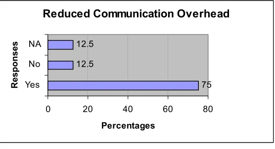
Figure 5.6 shows the results of the follow up survey. It is observed that 75% of the respondents agreed that communication overhead is reduced by making essential, low-level communication informal.

Reduced Communication Overhead

75 12.5

12.5

0 20 40 60 80

Yes No NA

Resp

o

n

ses

Percentages

FIGURE 5.6.REDUCED COMMUNICATION OVERHEAD To statistically analyze the survey results, we test the hypothesis that

HO: µ



reduction in communication overhead = µno reduction in communication overhead

= µno difference,

i.e. the null hypothesis (Ho) states that, the proportion of people who believe that there is a reduction in communication overhead and the proportion of people who believe that there is no reduction in communication overhead are equal. In other words, the null hypothesis states that pairing makes no difference to

communication overhead.

(60)

i.e. the alternative hypothesis states that the proportion of people who say that there is a reduction in communication overhead is greater than the proportion of people who say that pairing makes no difference to the communication overhead. Using normal approximation, we can reject the null hypothesis, HO, since there was a significant difference (p < .01).

The third question (see Appendix B) asked them to quantify the reduction in overhead due to pairing. We did not receive any definitive figures for the third question because 18 respondents refrained from answering this question. However, qualitatively, 12 respondents stated that the real benefit of pair communication comes from the improvement in the quality, not the quantity, of the communication.

5.6.3 Pair Rotation

The next survey question was aimed at understanding the teams’ use of pair rotation. The results indicated that pair rotation is widely practiced by the project teams. These results are displayed in Figure 5.7.There was a wide

consensus regarding the benefits of pair rotation with 94% of developers citing its use. For our statistical analysis purpose, we tested whether more than 50% of the people practiced pair rotation.

Pair Rotation

94 6

0 20 40 60 80 100

(61)

FIGURE 5.7.ADOPTION OF PAIR ROTATION

Thus we tested the hypothesis, HO: µ = 0.5

i.e. the null hypothesis states that the proportion of people who practice pair rotation is equal to 50%.

H1: µ > 0.5

i.e. the alternative hypothesis states that the proportion of people who practice pair rotation is greater than 50%

Using normal approximation, the p value of the test comes out to be a very small number (p < .01), thus we can reject the null hypothesis, HO. We can thus conclude that most teams practiced pair rotation.

In summary, the respondents consider pairing with an experienced mentor a very beneficial practice. Our analysis also indicates that there is also a

reduction in the communication overhead when pair programming is used. Lastly, we see that most teams that practice pair programming also practice pair rotation.

5.7 Subjective Responses

(62)

members. A few comments culled from the responses regarding pair programming and pair rotation indicate the views of the respondents

“…We start each iteration with assigned partners. Pairs are free to dynamically partner with whoever they need as they need. But, they always return to their assigned partner. We try very hard not to build “Towers of

Knowledge” in a single individual. So, it typically occurs that an assigned pair will seek out the person(s) that can help them, get the info, and get back to the

original pairing. Then they become more knowledgeable and will be sought after by other pairs. And so it goes.”

“… Pair programming (as other pair work) really allows newcomers to get concrete hands-on experience . . . and gives them rapid feedback and a quick learning by experience. Even when not proficient with the technology and task at hand, they can gain the feeling of contribution to working together with someone else.”

“…. We typically place responsibility for features on pairs of people and switch these pairs when the feature is completed. On the micro level, smaller tasks are performed on an ad hoc pairing basis (even though the responsibility for the feature still lies on the macro level).”

There are also “not-so-supportive” views on pair rotation. Quoting a response from the survey,

(63)

The above response suggests that one main reason could be that pairing also depends on the personality of the individual and the team. Our studies have demonstrated that, with most people, pair programming can produce

(64)

6. Pairing and Intercommunication

In this chapter we shall discuss with the help of illustrations the effect of pair programming on the intercommunication paths.

6.1 Communication Overhead

Communication overhead is defined as the average team member’s drop in productivity below his nominal productivity as a result of team communication [5]. Communication includes verbal communication, documentation, and any additional work required to build software. This additional work could involve, design reviews, coding, code reviews, or writing test cases. In any software development project, human communication is an essential component. It can also be viewed as part of the job, instead of overhead.

Brooks states, “If each part of the task must be separately coordinated with each other part, the effort increases as

where N= number of people in a team.

This mathematical equation models the nonlinear communication overhead of a team. Notice that the effort increases with the square of the number of people. [14].

Consider a case in which there are six solo developers working on

different but interrelated modules of a single application (n=6). Each programmer will interact with the other five programmers as shown in Figure 6.1. There are n*(n-1) / 2 or 15 communications paths between these six developers (n=6) and

(65)

these intricate and somewhat complex maze of intercommunication paths are definite contributors to communication overhead.

Communication paths = 6 * (6-1) / 2 = 15

FIGURE 6.1.INDIVIDUALS WORKING ON A TASK AND THE INTERCOMMUNICATION EFFORT

(N=6)

Consider the alternate case shown in Figure 6.2 in which these six

developers form three pairs; each pair working on double the number of modules than if they each worked alone. Because the each pair works intimately together to complete their shared modules, the communication overhead is significantly reduced. In this case there are (n)*(n-1)/2 or 3 communication paths between these three pairs (n=3). Pair rotations leads to an “on-the-spot” transfer of

Developer 1

Developer 2

Developer 3 Developer 5

Developer 6

(66)

information between the developers. The intercommunication overhead is significantly reduced.

Communication paths = 3 * (3-1) / 2 = 3

FIGURE 6.2.PAIRS WORKING ON A TASK AND THE INTERCOMMUNICATION EFFORT

Comparing Figure 6.1 and Figure 6.2, we observe how the complexity of the inter-group communication is significantly reduced. Pair programming enables fast and simple communication; it also reduces the number of

communication paths nonlinearly. Consider first if a team does not rotate pairs but assigns larger pieces of functionality to static pairs. Then, instead of breaking the project into n parts, the project is broken into (n/2) parts and the communication effort increase is reduced from n*(n-1)/2 to n*(n-2)/8. When pairs work together, they make decisions on dependencies, technical aspects, and interfaces as they design and implement code. No separate coordination

Pair 3 Pair 1

(67)

activities need occur; no dependencies and interfaces need special

documentation, improving the efficiency of team communication. If pairs do rotate, and programmers partner with the programmer with whom their task is interdependent, we believe this intercommunication cost can be even further reduced. Needed communication about interfaces and other issues will happen during the natural course of pairing. [8]

6.2 Our Hypothesis

(68)

7. Stutzke's Model Revisited

Chapter 4 discussed Brooks’ Law, which states that adding manpower to a late software project makes it later. Stutzke’s model explains in detail the process and costs of assimilating the additional manpower, including the diversion of their mentors from the project task itself. We considered a case where after a mid-project slip, the manpower was doubled and the original schedule was achieved. Stutzke offers valuable insights as to how workers should be added, trained, supported with tools, etc. so as to minimize the disruptive effects of adding them. His model predicts the additional manpower needed in order to complete the project on schedule.

Stutzke, however, also states that one important factor which has not been included in the Brooks’ model is that the new people must be team players in order for the predicted productivity gains to be realized. They must be willing to take directions and execute the process, which has been defined. They must not attempt to alter the process. Individuals must be disciplined and have a willingness to learn from others.

(69)

7.1 Our Survey Results

We will now revisit Stutzke’s model utilitizing new values obtained from our statistically significant survey results, as discussed in Chapter 6. Through this survey, we obtained the assimilation (a) and mentoring (m) values as follows:

a (with pairing) = 12 work-days = 12 * (365.25/ 250) = 17.5 calendar days a (without pairing) = 27 work-days

= 27 * (365.25/ 250) = 39.4 calendar days The value for mentoring time

m (with pairing) = 26% m (without pairing) = 36%

Effective assimilation time with paring a’= a (1+m)

= 12 * (1+ .26)

= 15.1 workdays or 22 calendar days. Effective assimilation time without paring

a’= a (1+m) = 27 * (1+ .36)

(70)

We know from Brooks’ Law Model, that the total effort expended assimilating the new staff is the sum of the students being mentored plus the effort of the existing staff that must mentor them as denoted by equation IV:

Ea = f*Ni*a + m*f*Ni*a = f*Ni*a*(1+m)

From our survey results, we observe that effective assimilation time a’ without pairing is 54 calendar days. Note: our non-pairing value for a’ is similar to Stutzke’s non-pairing value (58 calendar days. We found a’ with pairing is 22 calendar days. As explained in Chapter Four, Stutzke’s model was used to estimate the additional people required to complete the project on schedule. The model estimated that in order to complete the project within 121 work days (remaining time), the additional effort required was 8,863 person hours. Thus f = 8863 / (Ni * (1+ Overtime)* (r-a’)*8)), f=1.12. According to the model, in order to complete the project on time the project manager needs to more than double the staff (add 11 people). We shall calculate f using the reduced assimilation time due to pairing, thus,

f = Eadd / (Ni * (1+ Overtime)* (r-a’)*8))

= 8868 / (10 * 1.15* (121-15) * 8)

(71)

In Stutzke’s model, there is a limit on the number of new staff members that a mentor can train. We know from equation II, the useful effort delivered during assimilation = (1- f * m)* Ni. Thus, the useful effort delivered by the mentor during assimilation goes to zero as f Î 1/m. (Recall f = the fractional increase in staff) The maximum possible value of f is 1/m, since one existing staff person cannot train more than 1/m new staff members. Thus, m constrains f. Our studies indicate that pairing rotation removes this limit. It prevents

overloading of one mentor. The rotation allows the new team member to interact with different mentors.

The useful effort delivered to a project Eu, is given as,

Eu= sum of work delivered during the mentoring period (duration a) + work delivered after all the new staff members have been assimilated (duration of this period is r-a’, where r is the remaining time until project completion).

Eu= f * Ni * (r-a’) + Ni * r…Equation V

Our results show that the effective assimilation time and mentoring time is reduced due to pairing. Since assimilation is faster, more work can be achieved in the remaining days because (r-a’) is a larger number. Let us consider the effect of pairing on the net gain in the team’s output. The net gain in effort, Egain, is the difference between the useful effort (Eu) provided by adding the new staff and the effort which could have been provided by the original staff, is,

(72)

= f * Ni * (r – a’) >= 0

Thus, the first condition states that Egain is greater than zero if f > 0 i.e. some additional staff is added and r > a’ i.e. we must have enough time assimilate the new staff. From the above equation we observe that breakeven occurs when r = a’. No net gain is achieved unless r exceeds a’. The maximum total useful effort which can be delivered by adding more staff is Ni * (r-a’) / m. From our

observed results, the effective assimilation time (a’) is reduced due to pairing. This implies that breakeven occurs much earlier. Hence net gain is also achieved earlier than in a non-pairing environment.