Numerical Techniques for Hydrodynamic and Morphodynamic Modeling.

ABSTRACT

BERNSTEIN, ANDREW SCOTT. Numerical Techniques for Hydrodynamic and Morphody-namic Modeling. (Under the direction of Alina Chertock).

In this dissertation, we consider numerical techniques for modeling and computationally solving a hydrodynamic system, represented by the system of shallow water equations used to model the flows of coastal areas and rivers, and a morphodynamic system, represented by the shallow water equations with an Exner equation to govern sediment transport. We begin by deriving the equations for both the shallow water system and Exner equation from physical principles, and then we consider a number of formulations one can use to model the movement of sediment within the Exner equation. We then discuss finite volume methods and their use in solving systems of hyperbolic balance laws, particularly the shallow water equations with Exner equation.

In Part I, we implement a second-order central-upwind scheme for the 1-D shallow water equations with discontinuous bottom topography. The scheme is well-balanced, able to exactly numerically preserve a chosen steady state, and positivity preserving, ensuring that the height of the water never becomes negative which represents a non-physical state. This central-upwind scheme relies on a discontinuous piecewise linear reconstruction of the bottom topography function, and, thus, it is suitable for functions when the bottom contains large jumps and can be extended to models with moving, time-dependent bottom topography which will be studied in Part II. We then present the performance of the scheme, demonstrating the numerical scheme remains smooth while handling a small perturbation of steady state and accurately converging to the solution of a Riemann problem with both a unique solution or with multiple solutions.

Numerical Techniques for Hydrodynamic and Morphodynamic Modeling

by

Andrew Scott Bernstein

A dissertation submitted to the Graduate Faculty of North Carolina State University

in partial fulfillment of the requirements for the Degree of

Doctor of Philosophy

Applied Mathematics

Raleigh, North Carolina 2018

APPROVED BY:

Mansoor Haider Zhilin Li

Tien Khai Nguyen Alina Chertock

DEDICATION

BIOGRAPHY

ACKNOWLEDGEMENTS

I would like to thank my advisor, Dr. Alina Chertock, for all her support and guidance through-out my graduate career. I would also like to thank our collaborators, Dr. Alexander Kurganov for his contributions and insightful discussions as well as Dr. Tong Wu. Thank you to Dr. Gavin Conant, Dr. Mansoor Haider, Dr. Zhilin Li, and Dr. Khai Nguyen for serving on my dissertation committee and for your feedback and time and to the Mathematics Department at NC State for their financial support during my time at State.

TABLE OF CONTENTS

LIST OF TABLES . . . .viii

LIST OF FIGURES . . . ix

Chapter 1 INTRODUCTION . . . 1

1.1 Motivation . . . 1

1.2 Shallow Water Equations . . . 2

1.2.1 Derivation of First Equation: Conservation of Mass . . . 3

1.2.2 Derivation of Second and Third Equation: Conservation of Momentum . . 5

1.2.3 Hyperbolic System of Conservation and Balance Laws . . . 8

1.2.4 Steady States of Shallow Water Equations . . . 9

1.3 Sediment Transport Equation . . . 11

1.3.1 Derivation of Sediment Transport Equation . . . 12

1.3.2 Sediment Transport Formulations . . . 14

1.3.2.1 Du Boys (1879) . . . 15

1.3.2.2 Meyer-Peter-M¨uller (MPM) (1948) . . . 16

1.3.2.3 Fernandez Luque-VanBeek (FLV) (1976) . . . 17

1.3.2.4 Grass (1981) . . . 17

1.3.2.5 Nielsen (1992) . . . 17

1.3.2.6 Modified Grass (2012) . . . 17

1.4 Finite Volume Methods . . . 18

1.4.1 Alternatives to the Central-Upwind Scheme . . . 22

1.5 1-D Second Order Semi-Discrete Central-Upwind Scheme . . . 22

1.6 2-D Second Order Semi-Discrete Central-Upwind Scheme . . . 24

1.7 Outline of the Dissertation . . . 27

I Hydrodynamic: Shallow Water Equations with Discontinuous Bottom Topography 28 Chapter 2 A Well-Balanced, Positivity Preserving Central-Upwind Scheme for the 1-D Shallow Water System of Equations . . . 29

2.1 A Modified Second-Order Semi-Discrete Central-Upwind Scheme . . . 30

2.1.1 Reconstruction ofU . . . 31

2.1.2 Piecewise Linear Reconstruction of B . . . 32

2.1.3 Local Speeds of Propagation . . . 32

2.2 Well-Balanced Quadrature for the Geometric Source Terms . . . 32

2.3 Positivity Preserving Property . . . 34

2.3.1 Positivity Correction forw_e . . . 34

2.3.1.1 Velocity Desingularization . . . 35

2.3.2 Time Evolution and the Draining Time-Step . . . 35

2.4 Numerical Examples . . . 36

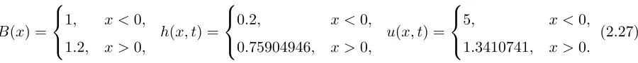
2.4.2 Example 2—Riemann Problem with Unique Solution . . . 37

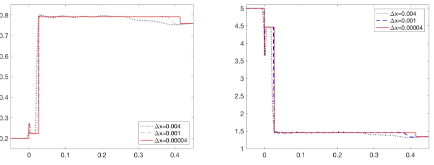
2.4.3 Example 3—Riemann Problem with Multiple Solutions . . . 39

2.5 Conclusion . . . 39

II Morphodynamic: Exner Equation to Govern Bed Load Sediment Transport 41 Chapter 3 1-D Shallow Water Equations with Exner Equation . . . 42

3.1 Eigenvalues for the Jacobian of the Shallow Water System with Exner Equation 43 3.2 Time Evolution . . . 45

3.2.1 Splitting Approach . . . 46

3.2.2 Non-Splitting Approach . . . 48

3.3 Spatial Discretization . . . 49

3.3.1 Non-Staggered Discretized Grid . . . 49

3.3.2 Staggered Discretized Grid . . . 49

3.4 Numerical Scheme for the Splitting Approach with the Bottom Evolved on a Non-Staggered Discretized Grid (S-NSG) . . . 51

3.4.1 Hydrodynamic Subsystem . . . 51

3.4.2 Morphodynamic Subsystem . . . 53

3.4.3 Time Evolution of S-NSG . . . 54

3.4.3.1 Time Evolution of S-NSG When the Splitting Time-Step Is Cho-sen Using the Morphodynamic Time-Step (S-NSG-M) . . . 55

3.4.3.2 Time Evolution of S-NSG When the Splitting Time-Step Is Cho-sen Using the Hydrodynamic Time-Step (S-NSG-H) . . . 56

3.5 Numerical Scheme for the Splitting Approach with the Bottom Evolved on a Staggered Discretized Grid (S-SG) . . . 56

3.5.1 Hydrodynamic Subsystem . . . 57

3.5.2 Morphodynamic Subsystem . . . 59

3.5.3 Time Evolution of S-SG . . . 61

3.5.3.1 Time Evolution of S-SG When the Splitting Time-Step Is Cho-sen Using the Morphodynamic Time-Step (S-SG-M) . . . 61

3.5.3.2 Time Evolution of S-SG When the Splitting Time-Step Is Cho-sen Using the Hydrodynamic Time-Step (S-SG-H) . . . 62

3.6 Numerical Scheme for the Non-Splitting Approach with the Bottom Evolved on a Non-Staggered Discretized Grid (NS-NSG) . . . 63

3.6.1 Time Evolution of NS-NSG . . . 65

3.7 Numerical Scheme for the Non-Splitting Approach with the Bottom Evolved on a Staggered Discretized Grid (NS-SG) . . . 65

3.7.1 Time Evolution of NS-SG. . . 69

3.8 Numerical Examples . . . 69

3.8.1 Example 1 – Comparison of Numerical Formulations . . . 69

3.8.2 Example 2 – Test of Order . . . 70

3.8.5 Example 5 – Sediment Mound Interacting Slowly with a Large Velocity

Water Flow . . . 75

3.8.6 Example 6 – Small Discontinuity in Sediment Bed . . . 76

3.9 Conclusion . . . 77

Chapter 4 2-D Shallow Water Equations with Exner Equation . . . 79

4.1 Eigenvaules for the Jacobian of the 2D Shallow Water System with Exner Equation 80 4.2 A Modified Second-Order Semi-Discrete Central-Upwind Scheme in Two Dimen-sions . . . 82

4.2.1 Numerical Fluxes . . . 83

4.2.2 Reconstruction . . . 85

4.2.3 Well-Balanced Quadrature for the Geometric Source Terms . . . 86

4.2.4 Local Speeds of Propagation . . . 87

4.2.5 Time Evolution . . . 87

4.3 Numerical Example in 2-D – Evolution of Conical Sediment Dune Interacting Slowly with the Water Flow . . . 87

4.4 Conclusion . . . 90

Chapter 5 Conclusions and Future Work . . . 91

References. . . 93

Appendices . . . .103

Appendix A Third Order Strong Stability Preserving Runge Kutta Method . . . 104

LIST OF TABLES

LIST OF FIGURES

Figure 1.1 Shallow Water Domain. . . 3 Figure 1.2 Left: Central (staggered) control volume. Right: Upwind control volume. . . 19 Figure 1.3 Central-Upwind Control Volume. . . 21 Figure 2.1 Example 1: Solution (w) computed by the well-balanced and non-well-balanced

central upwind schemes using N = 400 (top row) and N = 1600 (bottom row) uniform cells. Right column: zoom into the regionx∈[0.395,0.5]. . . . 38 Figure 2.2 Example 2: Solution (h on the left and u on the right) computed using

∆x= 0.004 and 0.001 and compared with the reference solution. . . 39 Figure 2.3 Example 3: Solution (h on the left and u on the right) computed by the

proposed central-upwind scheme using ∆x= 0.004, 0.001, and 0.00004. . . . 40 Figure 2.4 Example 3: Solution (h on the left and u on the right) computed by the

central-upwind scheme from [50] using ∆x= 0.004, 0.001, and 0.00004. . . . 40 Figure 3.1 Non-staggered discretized grid for U andB. . . 50 Figure 3.2 Staggered discretized grid consisting of U (blue) centered at the cell center

and ofB (black dashed) centered at the cell interface. . . 50 Figure 3.3 Example 1: Initial conditions att= 0 with N = 400. . . 70 Figure 3.4 Example 1: NS-SG, S-SG-M, and S-SG-H solutions (B) computed using N

= 400 att= 2.1. Right zoom into the regionx∈[0.8,1.4]. . . 71 Figure 3.5 Example 1: NS-NSG, S-NSG-M, and S-NSG-H solutions (B) computed using

N = 400 at t= 2.1. Right zoom into the regionx∈[1.0,1.25]. . . 71 Figure 3.6 Example 2: Solution (h in upper left, u in upper right, and B on bottom)

computed with N = 50, N = 100, N = 200,N = 400 att= 1.05. . . 73 Figure 3.7 Example 3: Solution (B) computed with N = 50, N = 100, N = 200,

N = 400, and approximate solution at t= 238709. . . 74 Figure 3.8 Example 4: Solutions (B) computed at t= 0 with N = 400 and at t = 238

with N = 100, N = 200, and N = 400 using water wave speed for the sediment (left) and using the sediment wave speed for the sediment (right). . 75 Figure 3.9 Example 5: Solution (B) computed with N = 400 at t= 1904. . . 76 Figure 3.10 Example 6: Solution (B) computed with N = 200 at t= 0 and t= 900000. . 77 Figure 4.1 Example 1: Approximate solution for the angle of spread. . . 88 Figure 4.2 Example 1: Solution (B) computed at t = 0 (left) and t = 360000 (right)

with ∆x= 50 and ∆y= 50. . . 89 Figure 4.3 Example 1: Solution (B) computed at t = 0 (left) and t = 360000 (right)

with ∆x= 50 and ∆y= 50. . . 89 Figure 4.4 Example 1: Evolution of Conical Dune (B) att= 0, t= 90000,t= 180000,

Chapter 1

INTRODUCTION

1.1

Motivation

In recent years the modeling of sediment transport has been of interest to those in the hydraulics community for its use in environmental and engineering problems. One example is that sediment transport can influence the construction of harbors since sediment entering the harbor can damage the layout of the harbor, and dredging the harbor can be expensive. In addition, sediment building up can cause reservoirs to lose a significant amount of their capacity. Looking at U.S. reservoirs in 1973, Cunge et al. [19] stated that, by 1973, 33% of the reservoirs built before 1935 had lost between 25% to 50% of their original capacity. The modeling of sediment transport can also be of use in the construction of underwater oil wells. Underwater oil wells, when built too low above the ocean floor, run the risk of sediment covering the wells. As a result, the wells are built taller than needed, a costly expenditure.

The modeling of sediment transport incorporates a balance between the modeling of flowing water and that of the sediment. The water flow is modeled using the Saint-Venant system of shallow water equations which was introduced over 140 years ago in [20] and is still used in modeling flow in rivers, lakes, and coastal areas. In this thesis, we use both the one-dimensional (1-D) and two-dimensional (2-D) Saint-Venant systems, with the 2-D system given as

       h hu hv        t +        hu

hu2+g₂h2 huv        x +        hv huv

hv2+g₂h2        y =        0 −ghBx

−ghBy

       , (1.1)

velocity in the y-direction and g is a constant for gravity.

Since the Saint-Venant system of shallow water equations (1.1) does not incorporate sed-iment and has a bottom B(x, y) that is independent of time, we use an additional equation to govern the sediment transport. Sediment transport is mainly characterized into two main categories: bed load transport and suspended load transport, which refer to the sediment on the bottom topography and sediment moving within the water column, respectively. If a model incorporates both of these processes, it is said to cover the total transport. A third category which is less commonly accounted for is saltation, which is when single grains jump a short distance over the bed, settling back onto it. This is a mixture of the bed load and suspension transport. Due to the complexity and different natures of the processes for bed load and sus-pended load transport many models focus on only one of these processes. In this thesis, we will not consider suspension load transport, instead focusing on bed load transport. For the transport of the sediment layer we will be using a bed load updating equation called an Exner equation [23] in 1-D and 2-D, with the 2-D Exner equation given by

Bt+ξ

∂qb1

∂x +ξ ∂qb2

∂y = 0, (1.2)

where the variable ξ = 1

1− is a constant with representing the porosity of the sediment layer. The closeris to zero the larger the particles that comprise the sediment. We also define qb1(h, u, v) to be the sediment transport discharge fluxes in the x-direction and qb2(h, u, v) to

be the sediment transport discharge fluxes in they-direction. These sediment fluxes depend on various water and sediment properties with a multitude of models used to represent them, a few of which are defined in Section 1.3.2.

1.2

Shallow Water Equations

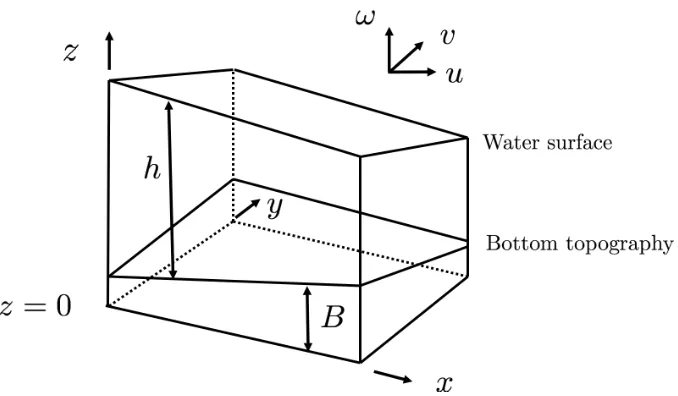
Figure 1.1: Shallow Water Domain.

1.2.1 Derivation of First Equation: Conservation of Mass

To balance the mass on a control volume Ω with boundary ∂Ω, we let ρ be the fluid density,

u∈_Rm _{be the fluid velocities, andnbe the outward normal vector on∂Ω. The balance of mass}

on a control volume Ω is given by ∂ ∂t

Z

Ω

ρ dV | {z }

The rate of change

of total mass in Ω

= − Z

∂Ω

(ρu)·n dA.

| {z }

The net mass flux across

the boundary of Ω

(1.3)

We can now apply the Divergence Theorem to the right hand side of (1.3) to rewrite the outward flux through the surface as the divergence over the region,

∂ ∂t

Z

Ω

ρ dV = − Z

Ω

∇ ·(ρu) dV. (1.4)

Assuming thatρ is smooth, we can move the derivative to the inside of the integral and rewrite (1.4) as

Z

Ω

∂ρ

∂t +∇ ·(ρu)

dV = 0. (1.5)

Since we chose our region Ω arbitrarily, we can rewrite (1.5) as ∂ρ

Equation (1.6) is a general formula for conservation of mass. In order to derive the con-servation of mass equation for the 2-D shallow water equations we need to apply boundary conditions at the bottomz=B(x, y) and the free surfacez=h(x, y, t) +B(x, y), recalling that in the shallow water equations the bottomB is fixed in time.

At the bottom z=B(x, y), we have

No normal flow: u∂B ∂x +v

∂B

∂y +ω = 0. (1.7)

At the surface the solution is slightly more complicated as the free surface may be moving. Therefore, at the free surfacez=h(x, y, t) +B(x, y), we have

No relative normal flow: ∂(h+B) ∂t +u

∂(h+B) ∂x +v

∂(h+B)

∂y −ω= 0. (1.8) We want depth averaged values for our equation, so we integrate (1.6) over the depth from z=B(x, y) to z=h(x, y, t) +B(x, y). Note for simplicity in our notation we will suppress the dependance onx,y, and t. Then,

Z h+B

B

∂ρ ∂t dz+

Z h+B

B

∇ ·(ρu) dz = 0, Z h+B

B

∂ρ ∂t dz+

Z h+B

B ∂(ρu) ∂x + ∂(ρv) ∂y + ∂(ρω) ∂z

dz = 0, Z h+B

B

∂ρ ∂t dz+

Z h+B

B ∂(ρu) ∂x + ∂(ρv) ∂y

dz+ (ρω)|_z=h+B−(ρω)|_z=B = 0. (1.9)

Since the functions that are being differentiated and the limits or integration are continuous and have continuous partial derivatives, we can apply the Leibniz integral rule to (1.9) to obtain

∂ ∂t

Z h+B

B

ρ dz −

ρ|z=h+B

∂(h+B)

∂t −ρ|z=B ∂B

∂t

+ ∂

∂x Z h+B

B

ρu dz−

ρu|_z=h+B∂(h+B)

∂x −ρu|z=B ∂B ∂x (1.10) + ∂ ∂y Z h+B

B

ρv dz−

ρv|_z=h+B∂(h+B)

∂y −ρv|z=B ∂B

∂y

+ ρω|_z=h+B−ρω|_z=B= 0.

and evaluating the remaining integrals, we have ∂

∂t(ρ(h+B)−ρB) + ∂

∂x(ρu(h+B)−ρuB) + ∂

∂y(ρv(h+B)−ρvB) = 0, ∂

∂t(ρh) + ∂

∂x(ρhu) + ∂

∂y(ρhv) = 0. (1.11) The density ρ depends on the pressure, temperature, and salinity of the fluid. We assume that the temperature and salinity are constant in our domain, and, since our fluid is water, it is incompressible. Therefore, ρ also does not depend on the pressure; thus, ρ can be taken as a constant. We factor ρ out of (1.11), and the first equation of the 2-D shallow water equation system is given by

∂

∂t(h) +∇ ·(hu) = 0. (1.12)

1.2.2 Derivation of Second and Third Equation: Conservation of Momentum To balance the momentum on a control volume Ω with boundary ∂Ω, we again let ρ be the fluid density, u∈_Rm _{be the fluid velocities, andn be the outward normal vector on ∂Ω. The}

balance of momentum on a control volume Ω is given by ∂

∂t Z

Ω

ρu dV | {z }

The rate of change

of total momentum in Ω

=− Z

∂Ω

(ρu)u·n dA

| {z }

The net momentum flux across

the boundary of Ω

+ Z

∂Ω

(pI−II)·n dA

| {z }

The surface forces

acting on∂Ω

+ Z

Ω

ρg dV, | {z }

The volume forces

acting on Ω

(1.13) wheregis the body force,pis the pressure,I is the identity matrix, andIIis the viscous stress tensor given by

II=       

τxx, τxy, τxz

τyx, τyy, τyz

τzx, τzy, τzz        . (1.14)

We can now combine the two surface integrals and apply the Divergence Theorem on them to get

∂ ∂t

Z

Ω

ρu dV = Z

Ω

∇ ·[(ρu)u+ρ(pI−II) +ρg] dV. (1.15) Assuming that ρ is smooth, we move the derivative to the inside of the integral, and rewrite (1.15) as

Z

Ω

∂(ρu)

∂t +∇ ·[(ρu)u+ (pI−II) +ρg]

Since we chose our region Ω arbitrarily, we can rewrite (1.16) as ∂(ρu)

∂t +∇ ·[(ρu)u+ (pI−II) +ρg] = 0. (1.17) Equation (1.17) is a general formula for conservation of momentum. In order to derive the equations specific to the 2-D shallow water equations we need to apply a few assumptions. The first is that the only body force acting on the system is the force of gravity. Thus g = (g1, g2, g3) ≡ (0,0,−g) where g is the acceleration due to gravity, a constant value. Secondly,

from the assumption that the vertical velocity is small and can be neglected, we have _DtDω =

∂ω

∂t +u· ∇ω = 0, where D

Dt denotes the total derivative which computes the time rate of change

of any quantity for a portion of material moving with a velocity u. Lastly, we assume that the flow is inviscid, meaning that the viscous stress tensor II is zero.

The system in (1.17) can now be written as        ρu ρv ρω        t +       

ρuu+p ρvu ρωu        x +        ρuv

ρvv+p ρωv        y +        ρuω ρvω

ρωω+p        z =        0 0 −ρg        . (1.18)

By expanding the derivatives in (1.18) and using the equation for conservation of mass (1.6), we rewrite (1.18) as

ρut+ρuux+ρvuy+ρωuz+px = 0, (1.19)

ρvt+ρuvx+ρvvy+ρωvz+py = 0, (1.20)

ρωt+ρuωx+ρvωy+ρωωz+pz = −ρg. (1.21)

Since we assume that the vertical velocity ω is small and thus the vertical component of accel-eration given by the material derivative _DtDω= 0, we can rewrite (1.21) as

ρωt+ρuωx+ρvωy+ρωωz+pz = −ρg,

ρDω

Dt +pz = −ρg,

pz = −ρg. (1.22)

At the free surface z = h+B, the pressure is equal to the pressure from the atmosphere, p =patm. For convenience we will takepatm to be zero. Now, integrating (1.22) and applying

the hydrostatic pressure relation

p=ρg[(h+B)−z], (1.23)

which represents the pressure exerted by a liquid. Note from (1.23) that the deeper you go under the surface, the greater the pressure will be. From the relation (1.23) we find a formula for the other pressure terms px and py in (1.19) and (1.20), respectively,

px = ρg(h+B)x, (1.24)

py = ρg(h+B)y. (1.25)

We further simplify (1.19) and (1.20), by noting thatpx and py are independent ofz, and thus

the left hand side must be as well. Therefore, thez velocity terms will vanish, andu andv are independent ofz. We rewrite (1.19) and (1.20), plugging in (1.24) and (1.25), to obtain

ρut+ρuux+ρvuy = −ρg(h+B)x, (1.26)

ρvt+ρuvx+ρvvy = −ρg(h+B)y. (1.27)

To express (1.26) and (1.27) in a conservative form similar to (1.11) for the conservation for mass, we rewrite the system, starting with (1.26), by first multiplying it by the fluid height h and adding (1.11) multiplied byu, to obtain

h(ρut+ρuux+ρvuy) +u(ρh)t+u(ρhu)x+u(ρhv)y = h(−ρg(h+B)x), (1.28)

(ρh)ut+u(ρh)t+ (ρhu)ux+u(ρhu)x+ (ρhv)uy+u(ρhv)y = −ρgh(h+B)x. (1.29)

As was stated with the conservation of mass equation,ρcan be taken as a constant and factored out. Once factored out, we separate the right hand side into thehx and Bx terms and rewrite

the left hand side, recognizing a number of chain rules. Thus, we have

hut+uht+ (hu)ux+u(hu)x+ (hv)uy+u(hv)y = −ghhx−ghBx, (1.30)

(hu)t+ (hu2)x+ (huv)y = −

1 2gh

2

x

−ghBx, (1.31)

(hu)t+ (hu2+

1 2gh

2₎

x+ (huv)y = −ghBx. (1.32)

Equation (1.32) represents the second of the 2-D shallow water equations: conservation of momentum in thex-direction.

adding (1.11) multiplied by v to obtain

h(ρvt+ρuvx+ρvvy) +v(ρh)t+v(ρhu)x+v(ρhv)y = h(−ρg(h+B)y), (1.33)

(ρh)vt+v(ρh)t+ (ρhv)ux+u(ρhv)x+ (ρhv)vy+v(ρhv)y = −ρgh(h+B)x. (1.34)

Again,ρcan be taken as a constant and factored out. Once factored out, we separate the right hand side into the hy and By terms and rewrite the left hand side, recognizing a number of

chain rules. Thus, we have

hvt+vht+ (hv)ux+u(hv)x+ (hv)vy+v(hv)y = −ghhy−ghBy, (1.35)

(hv)t+ (huv)x+ (hv2)y = −

1 2gh

2

y

−ghBy, (1.36)

(hv)t+ (huv)x+ (hv2+

1 2gh

2₎

y = −ghBy. (1.37)

Equation (1.37) represents the third of the 2-D shallow water equations: conservation of mo-mentum in they-direction.

1.2.3 Hyperbolic System of Conservation and Balance Laws

In the previous subsections, we derived the individual equations for the 2-D system of shallow water equations given by (1.12), (1.32), and (1.37), resulting in the system given in (1.1). The system of shallow water equations, belongs to the category of hyperbolic systems of the form,

∂

∂tU(x, y, t) + ∂

∂xF(U(x, y, t)) + ∂

∂yG(U(x, y, t)) =S(x, y, t). (1.38) In the general case,U∈_Rm _{is anm-dimensional vector of conserved variables, that is variables}

whose quantities are neither created nor destroyed. F(U) ∈_Rm _{and G(U) ∈}

Rm are referred

to as flux functions withS(x, y, t) being the source term. If the bottom topography is flat, then Bx = 0 and By = 0 in (1.1). Thus, S is zero, and a system written in the form of (1.38), is

called a conservation law when S(x, y, t) = 0. A conservation law in quasilinear form is given by

Ut+ ∂F ∂UUx+

∂G

∂UUy = 0, (1.39)

where ∂F ∂U,

∂G

∂U are Jacobian matrices of sizem×min the general case. We say the system of

conservation laws (1.39) is hyperbolic if any real combinationα∂F ∂U +β

∂G

∂U has real eigenvalues

and is diagonalizable.

energy, and thus can be modeled with PDEs of this form. Difficulties in solving these equations arise that are both inherent to the system and caused by solving the system numerically. The first difficulties may arise in solving (1.39) as the solutions to the system may have compli-cated structures such as shocks and rarefactions. Possible discontinuities in the solution may also develop in finite time, even if the initial conditions were smooth. Where the solution is discontinuous, the PDE is not satisfied in the classical sense, so we work with the integral form of the equations (1.5) and (1.16). A second difficulty, when dealing with the integral form of the system, is that we have weak solutions which are non-unique. Since the equations are only a model of reality, the challenge is to be able to choose a physically relevant solution.

When the source term in (1.38) is nonzero (S6= 0), the conservation laws are instead referred to as balance laws. Since most physical applications of the shallow water equations do not deal with a perfectly flat bottom where bottom derivatives are zero, they are usually represented as a balance law. This addition of a nonzero source term may make numerically solving the system a more complicated task. To help with numerically solving the balance laws a special set of solutions called steady-state solutions are used. These steady state solutions, which are solutions that do not change in time, i.e. their time derivatives are zero, are physically relevant and important for numerical methods. A good numerical method should be able to capture steady states and small perturbations of steady states. A numerical method which is able to capture a particular steady state is referred to as well balanced and will be further discussed section 1.4. In the following subsection, we will derive a formula for steady states of the shallow water equations.

1.2.4 Steady States of Shallow Water Equations

The 2-D system of shallow water equations (1.1) has both smooth and non-smooth steady state solutions. In this section, we derive some of these steady state solutions. At steady state all the time derivatives are zero, and therefore (1.1) reduces to

        

(hu)_x+ (hv)_y = 0, hu2+1₂gh2_x+ (huv)_y =−ghBx,

(huv)_x+ hv2+1₂gh2

y =−ghBy.

(1.40)

One solution to the first equation of (1.40) is (hu)_x = 0 and (hv)_y = 0. Since the spatial derivatives are both zero, this implies

Looking at the second equation of (1.40) we can expand using the chain rule to obtain

u(hu)x+ (hu)ux+ghhx+u(hv)y+ (hv)uy =−ghBx. (1.42)

From (1.41), we have that (hu)x = 0 and (hv)y = 0, and using this and rearranging (1.42) we

have

u

*0

(hu)x+ (hu)ux+ghhx+u

*0

(hv)y+ (hv)uy+ghBx = 0, (1.43)

h(uux+ghx+gBx+vuy) = 0, (1.44)

uux+ghx+gBx+vuy = 0. (1.45)

Since u is the velocity in thex-direction,uy = 0. Therefore, (1.45) can be rewritten as

uux+ghx+gBx+v

>

0

uy = 0, (1.46)

1 2u

2_+gh+gB

x

= 0, (1.47)

1 2u

2_+g(h+B)

x

= 0. (1.48)

Therefore, this implies that

1 2u

2_{+g(h+B) = constant. (1.49)}

We now consider the third equation of (1.40) which we expand using the chain rule to obtain v(hu)x+ (hu)vx+v(hv)y+ (hv)vy+ghhy+ =−ghBy. (1.50)

From (1.41) we have (hu)x = 0 and (hv)y = 0, and, using this and rearranging (1.50), we find

that

v

*0

(hu)x+ (hu)vy+v

*0

(hv)y+ (hv)vy+ghhy+ghBy = 0, (1.51)

h(uux+ghx+gBx+vuy) = 0, (1.52)

Since v is the velocity in they-direction we havevx = 0. Therefore, (1.53) can be rewritten as

u

>

0

vx+vvy+ghy+gBy = 0, (1.54)

1 2v

2_+gh+gB

y

= 0, (1.55)

1 2v

2_+g(h+B)

y

= 0. (1.56)

The third equation of (1.40) therefore implies that 1

2v

2_{+g(h+B) = constant. (1.57)}

Putting together equations (1.41), (1.48), and (1.56), the 2-D shallow water system (1.1) admits steady state solutions satisfying

hu= constant, hv = constant, 1

2u

2_{+g(h+B) = constant,}

1 2v

2_{+g(h+B) = constant.}

(1.58)

One of the most important steady states satisfying (1.58) is the stationary steady state, which is also called the ”lake-at-rest steady state”. This steady state describes a motionless lake and is satisfied when

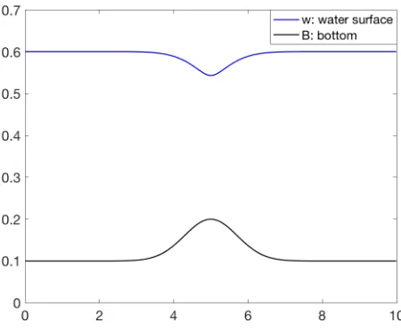
u= 0, v= 0, w:=h+B = constant, (1.59) wherew is defined to be the water surface.

1.3

Sediment Transport Equation

the mass transport of the sediment and will resemble the mass transport equation for the water (1.12). One main difference between the mass transport equation for the water and the Exner equation is that in (1.12) the water flux is always represented by hu in the x-direction and hv in the y-direction, while in (1.2) the sediment fluxes (qb1, qb2) in the Exner

equation can be represented by various formulations. These sediment flux formulations can depend on various physical parameters such as sediment grain size, and angle of elevation of the bottom topography. This will be discussed in Section 1.3.2 and examples can be found in [10, 30, 66, 67, 69, 75].

In sediment transport formulations, the mass of the sediment or total load for the sediment flux can be written in two parts that incorporate the bed load transport qb and the suspended

load transportqs. The bed load transport incorporates the sediment being transported on the

bed surface either by friction or gravity. The suspension transport incorporates the sediment that is picked up by the water and transported above the bed. The sediment moves within the water flow and may or may not be deposited back onto the bed. Thus we have that the total load for sediment flux is given by

qtot =qb+qs. (1.60)

While the total load sediment flux is made up of both the bed load and suspended sediment fluxes, one flux often dominates the other based on the environment. For slow moving water flows and beds with larger sediment, bed load transport will dominate as the water will not lift much sediment into the water flow. Suspended load transport will dominate in faster moving water flows and when the sediment is fine enough to be put into suspension. In a general, or typical, marine environment, bed load transport will dominate when sediment grains are coarser than approximately 0.2 mm, and suspended load transport will dominate for sediment grains finer than 0.2 mm [79].

In the following subsections, we derive the Exner equation for the sediment transport and discuss a number of empirically derived models for the sediment transport fluxes. These sedi-ment transport flux formulations are obtained using bed load transport sedisedi-ment fluxesqb.

1.3.1 Derivation of Sediment Transport Equation

The balance of sediment mass on a control volume Ω is then given by ∂

∂t Z

Ω

ρs(1−) dV

| {z }

The rate of change

of total mass in Ω

=− Z

∂Ω

[ρs(1−)ub]·n dA

| {z }

The net mass flux across

the boundary of Ω

, (1.61)

whereρs(1−) is the packing density andis the porosity of the sediment [19]. We now apply

the Divergence Theorem to the right hand side of (1.61), rewriting the outward flux through the surface to equal the divergence over the region,

∂ ∂t

Z

Ω

ρs(1−) dV =

Z

Ω

∇ ·[ρs(1−)ub] dV. (1.62)

Assuming thatρs(1−) is smooth, we can move the derivative to the inside and rewrite (1.62)

as

Z

Ω

∂[ρs(1−)]

∂t +∇ ·[ρs(1−)ub]

dV = 0. (1.63)

Since we chose our region Ω arbitrarily, we rewrite (1.63) as ∂[ρs(1−)]

∂t +∇ ·[ρs(1−)ub] = 0. (1.64) Equation (1.64) is a general formula for conservation of sediment mass. In order to derive the 2-D Exner equation for sediment mass transport, we need to apply boundary conditions at the bed level, z =B(x, y, t), where the sediment interacts with the water, and at the bottom topography reference level,z= 0, where the sediment is assumed to be fixed. In our boundary conditions, we assume the sediment is incompressible. Thus, ps is constant and the sediment

velocity is ub = (ub, vb, ωb) where ub, vb, and ωb are the sediment velocities in the x-direction,

y-direction andz-direction, respectively.

At the reference level z= 0, let the sediment velocity ub = (ub, vb, ωb). Then we have

ub=vb=ωb = 0. (1.65)

At the bed levelz=B(x, y, t), we have no relative normal flow, so ∂B

∂t +ub ∂B

∂x +vb ∂B

∂y +ωb= 0. (1.66)

dependance onx,y, and t. Then,

Z B

0

∂[ρs(1−)]

∂t dz+

Z B

0

∇ ·[ρs(1−)ub] dz = 0, Z B

0

∂[ρs(1−)]

∂t dz+

Z B

0

∂[ρs(1−)ub]

∂x +

∂[ρs(1−)vb]

∂y +

∂[ρs(1−)ωb]

∂z

dz = 0, Z B

0

∂[ρs(1−)]

∂t dz+

Z B

0

∂[ρs(1−)ub]

∂x +

∂[ρs(1−)vb]

∂y

dz

+ [ρs(1−)ωb]|z=B−[ρs(1−)ωb]|z=0 = 0.

(1.67) To simplify, we may factor outρs, since it is a constant by assumption, and apply the Leibniz

integral rule to (1.67) to obtain ∂ ∂t

Z B

0

(1−)dz − (1−)|z=B

∂B ∂t

+ ∂ ∂x

Z B

0

(1−)ub dz − (1−)ub|z=B

∂B ∂x

+ ∂ ∂y

Z B

0

(1−)vb dz − (1−)vb|z=B

∂B ∂y

+ ρω|z=B−ρω|z=0= 0. (1.68)

Using the boundary conditions given in (1.65) and (1.66), the evaluations at the boundaries in (1.68) equal zero. Canceling these terms and evaluating the remaining integrals results in

∂

∂t[(1−)B] + ∂ ∂xqb1+

∂

∂yqb2 = 0, ∂

∂tB+ξ ∂

∂xqb1+ξ ∂

∂yqb2 = 0. (1.69)

We recall that ξ = 1

1−, and we let qb1 =

RB

0 (1−)ub be the bed load sediment transport

flux in the x-direction, and qb2 =

RB

0 (1−)vb be the bed load sediment transport flux in the

y-direction. The values forqb1 andqb2 are not always straight forward and can be calculated in

a number of different ways. In the following sections, we will look at various ways of formulating the sediment transport flux.

1.3.2 Sediment Transport Formulations

This subsection discusses various formulations for the sediment transport fluxesqb = (qb1, qb2).

sediment transport fluxes. In general, hydrodynamic forcing agents, i.e the currents and waves, will affect the sediment movement primarily through the friction they exert on the sediment bed which is referred to as the bed shear stress τ0. Usually, τ0 can be written in terms of the

hydrodynamic unknowns as

τ0 =gρwRh|Sf|, (1.70)

wheregρwis the specific weight of the fluid,Rhis the hydraulic ratio which can be approximated

by h, and Sf is the friction term for Manning’s law given by

Sf =

gη2|u|u R_h4/3

, (1.71)

with η representing Manning’s coefficient. We then use τ0 to define the Shields parameter θ

(1936) which is a non-dimensional number used to calculate the initiation of sediment motion in a fluid. The Shields parameter is given by the following:

θ= τ0 g(ρs−ρw)d

, (1.72)

whereρs is the density of the sediment,ρw is the density of the fluid (in our case, water), and

dis the diameter of the sediment grains.

In addition, we make use of the threshold bed shear stress τcr and threshold Shields

pa-rameterθcr. The threshold or critical values are an indication of the amount of force required

before a sediment grain starts moving. Like the normal Shields parameter, the threshold Shields parameter is the ratio of the force exerted by the bed shear stress acting to move a grain of sediment and the submerged weight of the grain counteracting it given by the following formula:

θcr =

τcr

g(ρs−ρw)d

. (1.73)

Also note that we use the notationd50 to represent the size of a grain in the 50th percentile of

all the grains that make up the sediment.

1.3.2.1 Du Boys (1879)

The first sediment transport formula was proposed by Du Boys in 1879. Du Boys divided the sediment into nlayers with layer 1 being directly under the water, layer (n−1) directly above a fixed immobile bed, and layer n being the fixed bed. The thickness of the layers is assumed to bed50 with the velocity increasing linearly. If layer (n−1) starts moving with velocity ∆u,

with speed (n−1)∆u. We then have the total discharge per unit width is given by qb =

1

2(n−1)∆u(nd50). (1.74)

We now have a formula for qb, but the number of layers n is unknown, so we want to rewrite

this in terms of known quantities. To accomplish this, Du Boys used a tractive force method which says that the tractive forces or shear forces, moving a particle on the channel bed will not exceed those resisting the particle motion, i.e. shear stress of the flow is equivalent to the friction at the bed (τ0 =τcr). From the theory, we have

τ0 =θ(ρs−ρw)gnd50, (1.75)

where the friction is proportional to the submerged weight of the overlying grains. From our assumption of a tractive force method, there is only one layer (the immobile bed layer), son= 1 and τ0 =θ(ρs−ρw)gd50. Therefore, in general, when (n−1) layers are in motion τ0 =nτcr,

which impliesn= τ0

τcr. Plugging into (1.75), we obtain a formula for bed load sediment transport

given by

qb =

∆ud50

2τ2

cr

τ0(τ0−τcr). (1.76)

1.3.2.2 Meyer-Peter-M¨uller (MPM) (1948)

The MPM model is a well know empirical model proposed after a series of tests in Zurich in 1948 [67]. Meyer-Peter and M¨uller related bed load sediment flux and shear stress by the dimensionless formulation

qb = 8

s

ρs

ρw

−1

gd3_(θ−θ

cr)3/2. (1.77)

The MPM model is typically used for the transport of sediment in rocky rivers rather than sandy areas and assumes a flat bed. It is important to this model that the shear stress τ and the shield parameterθ are defined well as the (θ−θcr) term will prevent motion whileθ < θcr.

In the MPM model, we have θcr = 0.047 and d50= 0.4429 mm. However both these numbers

1.3.2.3 Fernandez Luque-VanBeek (FLV) (1976)

The FLV model proposed in 1976 [66] is an empirically derived model of a similar form to (1.77) given by

qb= 5.7

s

ρs

ρw

−1

gd3_(θ−θ

cr)3/2. (1.78)

In their experiments, FLV used smaller sediment particles, and introduced a downward slope of up to 22◦.

1.3.2.4 Grass (1981)

One of the simplest models derived for sediment flux was proposed by Grass in his book from 1981 [30]:

qb=Agukuk₂m−1, 1≤m≤4, (1.79)

where m= 3 is the usual value for the exponent. The value of A∈ [0,1] is an experimentally determined constant that takes into account the sediment properties such as the size of the sediment and the viscosity of the fluid. If A is zero, there is no sediment transport, and the system (1.1)-(1.2) reduces down to just the shallow water equations. WhenA is small, there is a weak interaction between the sediment and the water, and whenA is large (approaching 1), there is a strong interaction between the sediment and the water. One thing to note about this model is that there is no threshold necessary to initiate motion as there are in the other models in this section. This means that sediment bed load transport will begin with the fluid motion.

1.3.2.5 Nielsen (1992)

In 1992, Nielsen [69] proposed a model similar to that in (1.77) given by

qb = 12

s

ρs

ρw

−1

gd3_(θ−θ

cr)

√

θ, (1.80)

whereθcr = 0.05. This model is used for smaller grain sizes than the MPM model. 1.3.2.6 Modified Grass (2012)

and the water velocityu with what we will refer to as a Modified Grass model given by

qb =Adhukuk3₂, (1.81)

whereAd∈[0,1] is analogous toAin (1.79) and is an experimentally determined constant that

takes into account the sediment properties such as the size of the sediment and the viscosity of the fluid. Adding the water columnh to the flux helps fix a problem with Grass’s model that the maximum velocity on the free surface is where h = 0. This is not physically correct, as, when there is no water, there is nothing to move the sediment. Adding h to the sediment flux helps to correct this non-physical result, while allowing the flux to remain large at the bottom as expected when the problem is fully flooded.

1.4

Finite Volume Methods

In this section, we discuss finite volume methods and their use in solving hyperbolic systems of conservation and balance laws such as (1.39). In particular, we will discuss Godunov-type finite-volume projection-evolution methods which were first derived in [28]. With these methods, at each time level, a solution is globally approximated by a piecewise polynomial function, which is then evolved to a new time using the integral form of the system of hyperbolic conservation laws, and projected back onto the original grid. Numerical difficulties that may arise when solving (1.39) with finite volume methods include the possibility of complicated structures in the solutions, such as shocks and rarefactions, and discontinuities in the solution that can develop in finite time, even if the initial conditions are smooth. For simplicity, we will discuss the 1-D system of conservation laws given by

Ut+F(U)x =0, (1.82)

wherex∈Rm,t∈R+,U(x, t) is a vector of conserved quantities, andF(U) is a vector of flux

terms. The first step of the method is to divide the computational domain into non-overlapping intervals. For simplicity, we will divide our domain into uniform intervals called cells, where we denote Cj = (x_j−1

2, xj+ 1

2). Therefore, we have that xj+ 1 2 −xj−

1

2 = ∆x for allj. Second, if

an approximate solution is available at a time level tn, then we define cell averages to be the average of the integral of a cellj. Thus,

Un_j := 1 ∆x

Z

Cj

U(x, tn) dx. (1.83)

of the solution given by

e

Un_j(x) :=X

j

Un_jχCj, (1.84)

whereχCj is the characteristic function of the intervalCj. This reconstruction is only first order

accurate. In order to increase the accuracy, we would need to use a higher-order interpolant. A wide variety of reconstructions are available in literature, e.g. [1, 16, 27, 33, 34, 38, 42, 59]. We note that, in general, the solutions are discontinuous at the interfaces of the cells x = x_j±1

2.

Using the reconstructed interpolant as the initial data at time t =tn, we may now evolve to the next time level t=tn+1 by integrating (1.82) over Cj×[tn, tn+1]:

Ut = −F(U)x,

1 ∆x∆t

Z x

j+ 1₂

x

j−1

2

Z tn+1

tn

Utdxdt = −

1 ∆x∆t

Z x

j+ 1₂

x

j−1

2

Z tn+1

tn

F(U)xdxdt,

Un_j+1 = Un_j − 1 ∆x

Z tn+1

tn

h

F(U(x_j+1 2, t)

−F(U(x_j+1 2, t)

i

dt. (1.85)

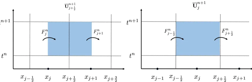
The way that (1.85) is calculated will depend on the space-time control volumes that are selected, as seen in Figure 1.2. The first finite volume upwind scheme was proposed by Godunov

Figure 1.2: Left: Central (staggered) control volume. Right: Upwind control volume.

in [28] in 1959. For upwind schemes, the computation cell is chosen such thatCj = (x_j−1 2, xj+

1 2).

Thus, the space-time control volume is given by h

x_j−1 2, xj+

1 2

i ×

tn, tn+1. To solve the upwind scheme, we need to be able to solve or exactly approximately the integrals for the fluxes in (1.85), since the solution U(x, tn) is discontinuous at the cell interfaces x = x_j±1

2 by the

nature of the reconstruction (1.84). In order to compute the required values at the interfaces

[4, 9, 16, 27, 28, 42, 59, 84]. The drawback to such schemes is that they are restricted to systems in which Riemann solvers exist, which can be computationally expensive and very hard to obtain analytically. However, if the Riemann solver is available, upwind schemes are highly accurate and less dissipative and diffusive than central schemes, resulting is less smearing at the discontinuities.

First-order central schemes were introduced in 1954 by Lax and Friedrichs [25, 56]. Within the finite volume framework, we will be working with central schemes which are staggered, referred to as central (staggered) schemes, which allow one to evolve the solution without solving Riemann problems exactly or approximately. This works by computing the cell averages over a centered grid that is staggered, given by computational cell C_j+1

2 = (xj, xj+1), rather

than the original computed grid centered at j. The central (staggered) schemes framework of being Riemann-problem-solver-free is of particular importance to solving multi-dimensional problems as Riemann problem solvers do not exist. Central schemes have been developed further in literature including staggered and non-staggered variants, multidimensional generalizations, and higher order methods, as seen in , e.g. [2, 6, 15, 39, 43, 50, 54, 60–62, 64, 65, 68, 71, 72].

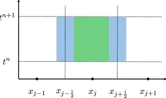
Figure 1.3: Central-Upwind Control Volume.

If the system from (1.82) does not have a zero right hand side, but instead is a balance law with a source termS(U) in 1-D given by

Ut+F(U)x=S(U), (1.86)

finding a solution is much more complicated. As discussed in section 1.2.3, one special class of solutions of particular importance to balance laws is that of steady states, or solutions that remain constant in time, since many additional solutions are small perturbations of steady states. Capturing these perturbations of steady state solutions can be numerically difficult, as the size of the perturbation may be smaller than the numerical error from the computation, particularly on a coarse grid. One way to overcome this challenge is to refine the grid, but this can be computationally expensive or unfeasible. Another difficulty that may arise is preserving the positivity of the computed solution so that it remains physically relevant as numerical oscillations may cause negative values for non-negative quantities. An example of this would be ensuring that the height of a water column is never negative, as the lowest it could be physically is zero which corresponds to the dry case.

1.4.1 Alternatives to the Central-Upwind Scheme

This thesis focuses on the development of second order semi-discrete central-upwind schemes in one and two dimensions which will be described fully in the following sections. However, we also wish to briefly discuss other schemes in literature used to solve the shallow water equations with Exner equation to govern sediment transport.

High resolution finite volume methods are used when high accuracy is needed such as when discontinuities and shocks are present. The computed solutions of these methods are second order or higher in accuracy at the smooth parts of the solution, are free of spurious oscillations, obtain high accuracy around discontinuities and shocks, and are computationally efficient. Two particular high resolution finite volume numerical schemes are Monotone Upstream-Centered Schemes for Conservation Laws (MUSCL), see Van Leer [85], and Weighted Essentially Non-Oscillatory (WENO), see Shu [78]. MUSCL schemes are a flux/slope limiter method which limit the solution gradient near shocks and discontinuities. When problems contain shocks and com-plex smooth solution structures, WENO schemes can provide good solution resolution around discontinuities and provide higher accuracy than second-order schemes. An implementation of a MUSCL method to the shallow water equations with Exner equation can be seen in [22] and an implementation of a WENO method to the shallow water equations with Exner equation can be seen in [35].

In addition to finite volume methods, finite element methods can be used in solving the shallow water equations with Exner equation. Finite element methods have the benefit that they can accommodate general cell shapes and thus can be well-suited for complex domains or topographical features [32]. One particular finite element method used is the Discontinuous Galerkin Method which combines the high-order accuracy and flexibility of elements of finite element methods with the local nature of finite volume methods. An implementation of a Discontinuous Galerkin Method to the shallow water equations with Exner equation can be seen in [83].

1.5

1-D Second Order Semi-Discrete Central-Upwind Scheme

In this section, we describe a 1-D second order semi-discrete central-upwind scheme for the hyperbolic balance law given by

Ut+F(U)x=S(U). (1.87)

First, the computational domain is broken into a uniform grid, for simplicity, with computational cells Cj := [x_j−1

2, xj+ 1

2] of size

C_j

central upwind scheme to (1.87) results in the following system of ordinary differential equations (ODEs):

d

dtUj(t) =−

H_j+1

2(t)−Hj− 1 2(t)

∆x +Sj(t), (1.88)

whereH_j±1

2 are the central-upwind numerical fluxes given by

H_j+1 2(t) =

a+

j+1₂F(U

−

j+1₂)−a

−

j+1₂F(U +

j+1₂)

a+

j+1₂ −a

−

j+1₂

+ a+

j+1₂a

−

j+1₂

a+

j+1₂ −a

−

j+1₂

U+ j+1₂ −U

−

j+1₂

, (1.89)

and the cell averages of the source term are given by

Sj(t)≈

1 ∆x

Z

Cj

S(U)dx. (1.90)

In (1.89),U±_j+1

2 are the left and right point values of the computed solution at the cell interface

x = x_j+1

2. For our scheme to be second-order, the point values should be calculated using

piecewise linear reconstructions given by

e

U(x) =X

j

Uj+ (Ux)j(x−xj)

·

χ

j(x), (1.91)

obtained at cell interfacesx=x_j+1 2 by

U+

j+1₂ =Uj+1−

∆x

2 (Ux)j+1, U −

j+1₂ =Uj+

∆x

2 (Ux)j. (1.92) In (1.91) and (1.92),

χ

j(x) is the characteristic function of the interval Cj and (Ux)j are the

numerical derivatives, which should be computed using a nonlinear limiter in order to minimize oscillations. In our numerical experiments shown in Chapter 2, 3, and 4, we use the generalized minmod limiter (see, e.g., [63, 68, 82, 85]):

(Ux)j = minmod

θUj−Uj−1

∆x ,

Uj+1−Uj−1

2∆x , θ

Uj+1−Uj

∆x

, θ∈[1,2], (1.93)

where the minmod function is defined by

minmod(z1, z2. . . ,) :=

        

minj{zj}, if zj >0 ∀j,

maxj{zj}, if zj <0 ∀j,

0, otherwise.

The parameter θ in (1.93) is used to control the amount of numerical viscosity with large θ values resulting in less dissipative results.

The one-sided local speeds of propagation a±

j+1₂ used in the central-upwind numerical flux

from (1.89) are obtained using the largest and smallest eigenvalues of the Jacobian matrix ∂F ∂U

whereλ1 < . . . < λN are the eigenvalues. Thus, we have

a+_j+1 2 = max λN ∂F

∂U(U

−

j+1 2

)

, λN

∂F

∂U(U

+

j+1 2 ) , 0 , a−

j+1₂ = min

λ1

∂F

∂U(U

−

j+1₂)

, λN

∂F

∂U(U

+

j+1₂)

, 0

.

(1.95)

Lastly, the evolution of the system of ODEs for the central-upwind semi-discretization system (1.88), should be integrated by a sufficiently accurate and stable ODE solver. We use a third order Strong Stability Preserving Runge Kutta (SSP-RK3) method from [29], which is outlined in Appendix A. In order for the computations to be stable, the time step should be chosen with the following CFL condition,

∆t≤δ ∆x max

j

a±

j+1₂

, δ≤ 1

2. (1.96)

1.6

2-D Second Order Semi-Discrete Central-Upwind Scheme

In this section, we describe a 2-D second order semi-discrete central-upwind scheme for the hyperbolic balance law given by

Ut+F(U)x+G(U)y =S(U). (1.97)

First, the computational domain is broken into a uniform grid in thex-direction andy-direction, for simplicity, with computational cells Cj,k :=

h x_j−1

2, xj+ 1 2

i

×hy_k−1 2, yk+

1 2

i

of size Cj,k

= ∆x∆y, centered at (xj, yk) for j = 1, . . . , N, k = 1, . . . , M with N and M being the number

of computational cells in the x-direction and y-direction, respectively. The cell averages are assumed to be known at a given timet and are computed by

Uj,k(t)≈

1 ∆x∆y

Z Z

Cj,k

Applying a second order semi-discrete formulation of the central upwind scheme to (1.98) results in the following system of ordinary differential equations (ODEs):

d

dtUj,k(t) =−

Hx_j+1

2,k(t)−H

x

j−1 2,k(t)

∆x −

Hy_j,k+1

2(t)−H

y

j,k−1 2(t)

∆y +Sj,k(t), (1.99) whereHx_j±1

2,k and H

y

j,k±1

2 are the central-upwind numerical fluxes given by

Hx_j+1

2,k(t) =

a+

j+1₂,kF(U

−

j+1₂,k)−a

−

j+1₂,kF(U

+

j+1₂,k)

a+

j+1₂,k−a

−

j+1₂,k

+ a+

j+1₂,ka

−

j+1₂,k

a+

j+1₂,k−a

−

j+1₂,k

U+

j+1₂,k−U

−

j+1₂,k

,

Hy_j,k+1 2(t) =

b+_j,k+1 2

G(U−_j,k+1 2

)−b−_j,k+1 2

G(U+_j,k+1 2

) b+_j,k+1

2

−b−_j,k+1 2

+

b+_j,k+1 2

b−_j,k+1 2

b+_j,k+1 2

−b−_j,k+1 2

U+

j,k+1₂ −U

−

j,k+1₂

,

(1.100) and the cell averages of the source term are given by

Sj,k(t)≈ 1 ∆x∆y

Z Z

Cj,k

S(U)dxdy. (1.101)

In (1.100), U±_j+1

2,k and U

±

j,k+1₂ are the left and right point values and bottom and top

point values, respectively, of the computed solution at the cell interface x=x_j+1

2, y =yk and

x = xj, y = y_k+1

2. For our scheme to be second-order the point values should be calculated

using piecewise linear reconstructions given by

e

U(x, y) =X

j,k

Uj,k+ (Ux)j,k(x−xj) + (Uy)j,k(y−yk)

·

χ

j,k(x, y), (1.102)

obtained at the midpoint cell interfacesx_j±1 2, yk

, and xj, yk±1 2

by

U+_j+1 2,k

=Uj+1,k−

∆x

2 (Ux)j+1,k, U −

j+1 2,k

=Uj,k+∆x

2 (Ux)j,k,

U+_j,k+1 2

=Uj,k+1−

∆y

2 (Uy)j,k+1, U −

j,k+1 2

=Uj,k+∆y

2 (Uy)j,k. (1.103) In (1.102) and (1.103),

χ

j,k(x, y) is the characteristic function of the intervalCj,k and (Ux)j,k

1-D case in Section 1.5, we use the generalized minmod limiter:

(Ux)j,k = minmod

θUj,k−Uj−1,k

∆x ,

Uj+1,k−Uj−1,k

2∆x , θ

Uj+1,k−Uj,k

∆x

, θ∈[1,2], (1.104)

(Uy)j,k = minmod

θUj,k−Uj,k−1

∆y ,

Uj,k+1−Uj,k−1

2∆y , θ

Uj,k+1−Uj,k

∆y

, θ∈[1,2], (1.105) where the minmod function is defined by

minmod(z1,1, . . . , zj,k) :=

        

minj,k{zj,k}, if zj,k >0 ∀j, k,

maxj,k{zj,k}, if zj,k <0 ∀j, k,

0, otherwise.

(1.106)

The parameter θ in (1.104) and (1.105) is used to control the amount of numerical viscosity with largeθ values resulting in less dissipative results.

The one-sided local speeds of propagation in the x-direction and y-direction, a±

j+1₂,k and

b±

j,k+1₂, used in the central-upwind numerical flux from (1.100) are obtained using the largest and

smallest eigenvalues of the Jacobian matrices ∂F ∂U and

∂G

∂U, respectively, whereλ1 < . . . < λN

are the eigenvalues. Thus, we have

a+

j+1₂,k = max

λN

∂F

∂U(U

−

j+1₂,k)

, λN

∂F

∂U(U

+

j+1₂,k)

, 0

,

a−

j+1₂,k = min

λ1

∂F

∂U(U

−

j+1₂,k)

, λ1

∂F

∂U(U

+

j+1₂,k)

, 0

,

b+_j,k+1 2 = max λM ∂G

∂U(U

−

j,k+1 2

)

, λM

∂F

∂U(U

+

j+1 2 ) , 0 , b−

j,k+1₂ = min

λ1

∂G

∂U(U

−

j,k+1₂)

, λ1

∂F

∂U(U

+

j,k+1₂)

, 0

.

(1.107)

Lastly, the evolution of the system of ODEs for the central-upwind semi-discretization sys-tem (1.99), should be integrated by a sufficiently accurate and stable ODE Solver. We use a third order Strong Stability Preserving Runge Kutta (SSP-RK3) method from [29], which is outlined in Appendix A. In order for the computations to be stable, the time step should be chosen with the following CFL condition:

∆t≤δmin ∆x max j a±

j+1₂,k

, ∆x max j b±

j,k+1₂

, δ ≤ 1

1.7

Outline of the Dissertation

Part I

Hydrodynamic: Shallow Water

Equations with Discontinuous

Chapter 2

A Well-Balanced, Positivity

Preserving Central-Upwind Scheme

for the 1-D Shallow Water System of

Equations

The contents of this chapter have been submitted to the Bulletin of the Brazilian Mathematical

Society [5].

2.1

A Modified Second-Order Semi-Discrete Central-Upwind

Scheme

To start, the 1-D system of shallow water equations can written from (1.12) and (1.32) by letting u= (u,0,0)>, resulting in

   h hu    t +    hu

hu2+1₂gh2    x =    0 −ghBx

 

. (2.1)

In Section 2.2, we discuss how to build the numerical scheme to be well balanced, by exactly preserving the lake-at-rest steady state (1.59). To this end, we choose to work with equilibrium variables, which remain fixed at our chosen steady state. From (1.59) and the first equation of (1.58), two such variables are the water surface w = h+B and the discharge q = hu. Following [50], we start by rewriting the system (2.1) in terms of the equilibrium variables

U= (w, q)>:

   w q    t +    q q2 w−B +

g

2(w−B)

2    x =    0 −g(w−B)Bx

 

. (2.2)

Furthermore, we expand and rewrite the second equation in (2.2) to make it easier to work with in Section 2.2. System (2.2) then becomes,

   w q    t +    q q2

w−B+

g 2(w

2_−2wB)

   x =    0 −gwBx

 

. (2.3)

We introduce a uniform grid xα := α∆x with a finite volume cell denoted by Cj :=

[x_j−1 2, xj+

1

2], in which a cell average of the computed solution,

Uj(t)≈

1 ∆x

Z

Cj

U(x, t)dx, (2.4)

is assumed to be known at a given time t. The cell averages are evolved in time based on the following equation:

d

dtUj(t) =−

H_j+1 2(t)

−H_j−1 2(t)

whereH_j±1

2 are the central-upwind numerical fluxes from [45] given by

H_j+1 2(t) =

a+

j+1₂F(U

−

j+1₂, B

−

j+1₂)−a

−

j+1₂F(U +

j+1₂, B +

j+1₂)

a+

j+1₂ −a

−

j+1₂

+ a+

j+1₂a

−

j+1₂

a+

j+1₂ −a

−

j+1₂

U+ j+1₂ −U

−

j+1₂

, (2.6)

withF(U, B) :=

q, qu+g 2(w

2_−2wB)>_{. Note, that, in contrast to the general central-upwind}

scheme in (1.5) and the numerical scheme from [50], the numerical fluxes now make use ofB± which are the left and right point values of the computed solution at the cell interfacex=x_j+1

2.

The cell averages of the geometric source term are given by

Sj(t)≈

1 ∆x

Z

Cj

S(U, B)dx. (2.7)

where S = (0,−gwBx)>. For the rest of this chapter, we will drop the notation t for time

dependence for simplicity where it is appropriate. The construction of the numerical scheme will be complete once the numerical fluxes inH_j±1

2 in (2.6) and the source termSj in (2.7) are

computed such that the resulting method is well-balanced and positivity preserving. 2.1.1 Reconstruction of U

In equation (2.6),U±_j+1

2 are the left and right point values of the computed solution at the cell

interface x =x_j+1

2. For our scheme to be second-order, the point values should be calculated

using piecewise linear reconstructions

e

U(x) =X

j

Uj+ (Ux)j(x−xj)

·

χ

j(x), (2.8)

obtained at cell interfacesx=x_j+1 2 by

U+

j+1₂ =Uj+1−

∆x

2 (Ux)j+1, U −

j+1₂ =Uj+

∆x

2 (Ux)j. (2.9) In (2.8) and (2.9), recall,

χ

j(x) is the characteristic function of the interval Cj, and (Ux)j

2.1.2 Piecewise Linear Reconstruction of B

The primary differences in our numerical scheme to the central-upwind scheme in [50] stem from our use of a generally piecewise discontinuous linear reconstruction for the bottom topography B instead of a continuous piecewise linear approximation. This reconstruction is obtained using the same generally piecewise discontinuous linear reconstruction as in (2.8) and (2.9) given by

e

B(x) =X

j

[B(xj) + (Bx)j(x−xj)]·

χ

to obtain the point values B±

j+1₂ atx=xj+12:

B+

j+1₂ =Bj+1−

∆x

2 (Bx)j+1, B −

j+1₂ =Bj+

∆x

2 (Bx)j. (2.11) 2.1.3 Local Speeds of Propagation

The one-sided local speeds of propagationa±_j+1 2

used in the central-upwind numerical flux (2.6) are obtained from the largest and smallest eigenvalues of the Jacobian matrix ∂F

∂U given by

∂F

∂U =

  

0 1

−_(w−q2_B)2 +

g

2(2w−wB)

2q w−B

 

. (2.12)

The characteristic equation reduces toλ2_−2uλ+u2_{−gh= 0, which can be solved analytically}

to obtain the eigenvaluesλ1 =u+

√

ghandλ2=u−

√

gh. Thus, the one-sided local speeds of propagation are

a+

j+1₂ = max

u+

j+1₂ +

r gh+

j+1₂ , u

−

j+1₂ +

r gh−

j+1₂ , 0

,

a−

j+1₂ = min

u+

j+1₂ −

r gh+

j+1₂ , u

−

j+1₂ −

r gh−

j+1₂ , 0

.

(2.13)

2.2

Well-Balanced Quadrature for the Geometric Source Terms

fluxes and source term. The numerical fluxes at the discrete level are given by: H(2)

j+1₂ −H (2)

j−1 2 ∆x = 1 ∆x  

a+h(_wq₋2_B)−+g 1₂w2−wB−i−a−h(_wq₋2_B)++g 1₂w2−wB+i a+_−a−

 

j+1₂

+ a+

j+1₂a

−

j+1₂

a+

j+1₂ −a

−

j+1₂

q+−q−_j+1 2

− 1 ∆x

 

a+h(_wq₋2_B)−+g 1₂w2−wB−i

−a−h(_wq₋2_B)++g 1₂w2−wB+i a+_−a−

 

j−1₂ +

a+

j−1 2

a−

j−1 2

a+

j−1 2

−a−

j−1 2

q+−q−_j−1 2

. (2.14)

Since q is a constant zero,q±

j+1₂ =q

±

j−1 2

= 0. Applying this condition to (2.14), we have

H(2)

j+1₂ −H (2)

j−1 2 ∆x = 1 ∆x       a+ " ( * 0 q2

w−B)

−_+g 1 2w

2_−wB− #

−a− " * 0

(_wq₋2_B)++g 1₂w2−wB+ #

a+_−a−

     

j+1 2

+ a+

j+1₂a

−

j+1₂

a+

j+1₂ −a

−

j+1₂

:0

q+−q−_j+1 2 − 1 ∆x       a+ " *0

(_wq₋2_B)−+g 1₂w2−wB− #

−a− "

*0

(_wq₋2_B)++g 1₂w2−wB+ #

a+_−a−

     

j−1 2

+ a+

j−1₂a −

j−1₂ a+_j−1

2

−a−_j−1 2

:

0

q+−q−

j−1 2