University of South Carolina
Scholar Commons
Theses and Dissertations
2018
Understanding Early Amyloid-ß Aggregation to
Engineer Polyacid-Functionalized Nanoparticles as
an Inhibitor Design Platform
Nicholas Vander Munnik
University of South CarolinaFollow this and additional works at:https://scholarcommons.sc.edu/etd
Part of theChemical Engineering Commons
This Open Access Dissertation is brought to you by Scholar Commons. It has been accepted for inclusion in Theses and Dissertations by an authorized administrator of Scholar Commons. For more information, please [email protected].
Recommended Citation
Understanding Early Amyloid-β Aggregation to Engineer Polyacid-Functionalized Nanoparticles as an Inhibitor Design
Platform
by
Nicholas Van der Munnik
Bachelor of Science Clarkson University 2013
Submitted in Partial Fulfillment of the Requirements
for the Degree of Doctor of Philosophy in
Chemical Engineering
College of Engineering and Computing
University of South Carolina
2018
Accepted by:
Mark J. Uline, Major Professor
Melissa A. Moss, Major Professor
Jochen Lauterbach, Committee Member
Andrew Greytak, Committee Member
John Weidner, Committee Member
c
Copyright by Nicholas Van der Munnik, 2018
Abstract
Alzheimer’s disease (AD) is characterized by the presence of amyloid-β (Aβ)
pro-tein aggregates in the brains of those afflicted. This propro-tein aggregates via a complex
pathway to progress from monomers to soluble oligomers and ultimately insoluble
fib-rils. Due to the dynamic nature of aggregation, it has proven exceedingly difficult to
determine the precise interactions that lead to the formation of transient oligomers.
A statistical thermodynamic model has been developed to elucidate these
interac-tions. Aβ was simulated using fully-atomistic replica exchange molecular dynamics.
We use an ensemble of 5×10⁵ configurations taken from these simulations as input
for a self-consistent field theory (SCFT) that explicitly accounts for the size, shape
and charge distribution of the amino acids comprising Aβ as well as all molecular
species present in solution. The solution of the model equations provides a prediction
of the probabilities of the configurations of the interacting Aβmonomers and the
po-tential of mean force between two monomers during the dimerization process. This
model constitutes a powerful methodology to elucidate the underlying physics of the
Aβ dimerization process as a function of pH, temperature and salt concentration.
Gold nanoparticles (NPs) are a promising class of materials for medical
applica-tions due to the unique properties that particles in this size range have on biological
systems. Moreover, these NPs can be functionalized with ligands to effect a veritable
cornucopia of biological responses. We have performed a central composite design of
experiment to determine the effects of NP size and the length of end-grafted
poly-acrylic acid (PAA) molecules on the aggregation of Aβ. We find that a complex
that is dependent on the bulk ion concentration. In particular, a regression
anal-ysis of the measured data indicates that NP diameter is negatively correlated with
Aβ aggregation lag time and that an optimum length of PAA exists at low ion
con-centrations with respect to this response. We develop another SCFT to model the
behavior of the PAA on the NPs’ surface. We present this theory with two distinct
formulations each employing a different polymer model and discuss the implications
and practicality of their respective use. These theories allow us to make
predic-tions regarding the effects that the polymers have on local solution condipredic-tions as a
function of the same bulk solution conditions that modulate Aβ aggregation and to
put our experimental observations in a more general theoretical context. The
ca-pacity to synthesize, characterize and test the efficacy of PAA-functionalized NPs as
Aβ aggregation inhibitors coupled with accurate theoretical modeling of the
thermo-dynamics and molecular organization of the system at the nanoscale constitutes a
Table of Contents
Abstract . . . iii
List of Tables . . . vii
List of Figures . . . viii
List of Symbols . . . xii
List of Abbreviations . . . xv
Chapter 1 Introduction . . . 1
1.1 The Specter of Alzheimer’s Disease . . . 1
1.2 Amyloid-β Oligomers: The Elusive Culprit . . . 3
1.3 The Fashionable and Wrong Tool for the Job . . . 6
Chapter 2 Statistical Thermodynamics of AβOligomer Inter-actions . . . 10
2.1 Background . . . 10
2.2 Theoretical Methodogy . . . 11
2.3 Theoretical Results . . . 23
2.4 Discussion of Theoretical Predictions . . . 29
Chapter 3 Nanoparticle Systems as an Alzheimer’s Disease
Ther-apeutic Platform . . . 37
3.1 Background . . . 37
3.2 Experimental Methods . . . 39
3.3 Experimental Results and Discussion . . . 59
3.4 Self-Consistent Field Theory for Polyacid-Functionalized Nanoparticles 67 3.5 Reflections on the Methodology and Future Work . . . 90
Chapter 4 Conclusions and Future Work . . . 92
Bibliography . . . 96
Appendix A Additional Analysis of Aβ Model . . . 107
A.1 Excluded Volume Interactions . . . 107
List of Tables
Table 2.1 Extrema of PMF and MF . . . 27
Table 3.1 AuNPs for Thermal Citrate Method . . . 45
Table 3.2 AuNPs for Reverse Thermal Citrate Method . . . 46
Table 3.3 AuNPs from Citrate/NaBH4 Method . . . 48
Table 3.4 ptBA Samples from RAFT Polymerization . . . 50
List of Figures
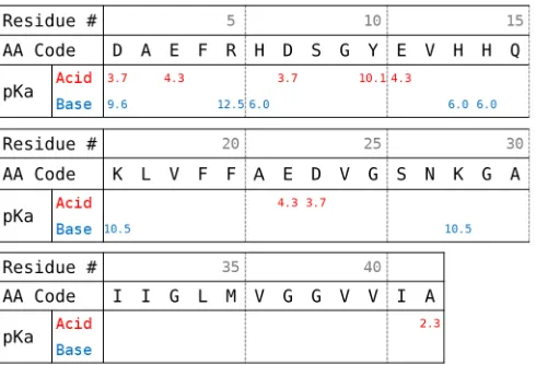
Figure 2.1 Amino acid sequence and pKa values for chemical equilibrium
sites of Aβ1−42. pKa’s for acidic and basic sites are shown in
red and blue, respectively. . . 11
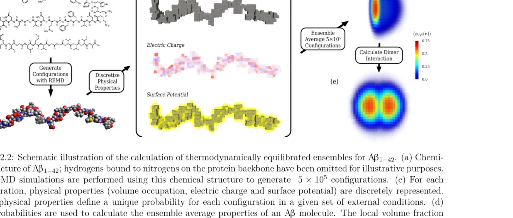
Figure 2.2 Schematic illustration of the calculation of thermodynamically
equilibrated ensembles for Aβ1−42. (a) Chemical structure of
Aβ1−42; hydrogens bound to nitrogens on the protein backbone
have been omitted for illustrative purposes. (b) REMD sim-ulations are performed using this chemical structure to
gener-ate 5×10⁵ configurations. (c) For each configuration, physical
properties (volume occupation, electric charge and surface po-tential) are discretely represented. These physical properties define a unique probability for each configuration in a given set of external conditions. (d) Said probabilities are used to
calcu-late the ensemble average properties of an Aβ molecule. The
local volume fraction of an Aβensemble is plotted according to
the color scale on the right. (e) By constraining the centers of
mass of two Aβ molecules to different relative separations, the
potential of mean force (PMF) is determined. . . 12
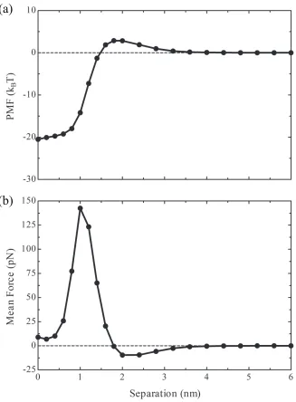
Figure 2.3 Potential of mean force (PMF) inkBT (a) and mean force (MF)
in pN (b) for two interacting Aβ1−42molecules calculated at pH
8, 150 mM NaCl and 25◦C,Condition 1. A potential or force of
0 has been defined as that which exists for two isolated Aβ1−42
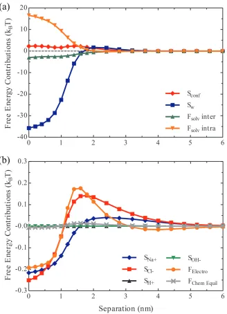
Figure 2.4 Individual free energy contributions to the PMF acting
be-tween two Aβ1−42 molecules at pH 8, 150 mM NaCl and 25
◦C, Condition 1. (a) Free energy terms with contributions to
the PMF including the configurational entropy of the Aβ1−42
molecules (red diamonds), the translational entropy of the wa-ter (blue squares), the intramolecular free energy of solvation (green up triangles) and the intermolecular free energy of sol-vation (orange down triangles). (b) Free energy terms with smaller contributions to the potential of mean force (MF),
in-cluding the translational entropies of N a+ (blue diamonds),
Cl− (red squares), H+ (black up triangles) and OH− (green
down triangles) as well as the electrostatic free energy (orange
circles) and the free energy of chemical equilibrium (gray times). . 26
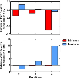
Figure 2.5 Deviations of extrema for PMF and MF from those calculated
at pH 8, 150 mM NaCl and 25◦C, Condition 1. . . 28
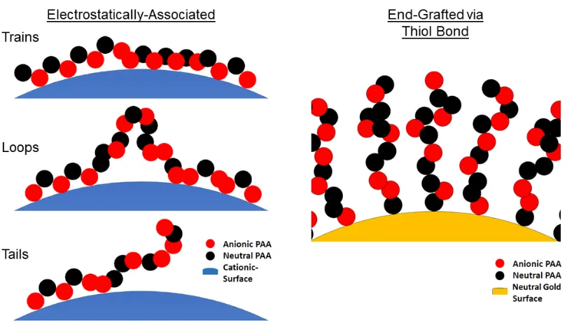
Figure 3.1 Illustration of disparate molecule architectures for
electrostatically-associated polyacid layers vs. end-grafted binding motifs. . . 41
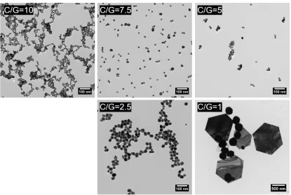
Figure 3.2 TEM micrographs showing size and morphology of AuNPs
syn-thesized with thermal citrate methodology and varied C/G ra-tio. The author would like to acknowledge Kate Mingle for
taking the TEM images. . . 44
Figure 3.3 TEM micrographs showing size and morphology of AuNPs
syn-thesized with reverse thermal citrate methodology and varied C/G ratio. The author would like to acknowledge Kathleen
Mingle for taking the TEM images. . . 46
Figure 3.4 TEM micrographs showing size and morphology of AuNPs
syn-thesized with citrate and NaBH4 at room temperature. The
author would like to acknowledge Kathleen Mingle for taking
the TEM images. . . 48
Figure 3.5 Number of tBA repeat units (N) in pTBA samples prepared
with RAFT polymerization and varied tBA/CTA ratios. The
Figure 3.6 DLS determination of hydrodynamic diameter of 5.98±0.18 nm AuNPs a) as synthesized/citrate capped and b) capped with 35.8 repeat unit PAA. The author would like to acknowledge
Kathleen Mingle for performing the DLS experiments. . . 53
Figure 3.7 TGA profile of PAA-AuNPs. The author would like to
acknowl-edge Kathleen Mingle for performing the TGA experiment. . . 54
Figure 3.8 TEM images of selected AuNPs for central composite design. . . . 55
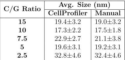
Figure 3.9 Size distributions generated with CellProfiler of selected AuNPs
for Aβaggregation experiments. . . 55
Figure 3.10 CCD of PAA-functionalized NPs with degree of PAA
polymer-ization N plotted versus NP core diamater D. Experimentally
measured points are plotted as gray circles with horizontal error
bars indicating standard deviation ofD and vertical error bars
indicating PDI of PAA. Open red circles indicate design points
used for analysis of experimental results. . . 57
Figure 3.11 Layout of 96 well plate for Aβ aggregation assays. NP sample
numbers are shown in their respective wells. . . 58
Figure 3.12 Lag time determination for sample aggregation data. Lag time is defined as the time at which tangent of the point with the greatest time derivative of flourescence intersects the baseline
flourescence. . . 59
Figure 3.13 Lag extension factor for the nine NP samples of the CCD. Blue, unpatterned bars represent lag extension factor for the 0 mM NaCl while red, dotted bars indicate that for 150 mM NaCl. Both data sets were obtained at pH 8.0. Error bars represent
the standard error of the mean. . . 60
Figure 3.14 Contour plots of degree of polymerization (N) versus NP
diam-eter (D) for the regression analysis of the NP CCD data. In
these plots, the model predictions for lag extension factor are rendered different colors according to the color bar at right. The top subplot shows the regression model for 0 mM NaCl while the bottom subplot shows that for 150 mM NaCl. Both data sets were obtained at pH 8.0. Design points are represented by
Figure 3.15 Volume fractions of molecular species as a function of distance from the NP surface calculated using the RIS chain model. Both plots show these results for a NP with a diameter of 14.5 nm, a degree of polymerization of PAA of 11 and a PAA grafting
density of 0.58 nm−2. Both plots have been calculated for a
bulk pH of 8.0 and a temperature of 25◦C. Panel A shows the
volume fractions for the case of a bulk concentration of 0 mM
NaCl and Panel B for 150 mM NaCl. . . 74
Figure 3.16 pH as a function of distance from the NP surface calculated using the RIS chain model. pH functions were calculated for a bulk pH of 8.0 (indicated by a dotted line) and a temperature
of 25◦C. . . 75
Figure 3.17 Volume fractions of molecular species as a function of distance from the NP surface calculated using the continuous Gaussian chain model for a NP with a diameter of 14.5 nm, a degree of polymerization of PAA of 11 and a PAA grafting density of
0.58 nm−2. This plot has been calculated for a bulk pH of 8.0,
a temperature of 25 ◦C and a bulk concenctration of 150 mM NaCl. 89
Figure 3.18 pH as a function of distance from the NP surface calculated using the continuous Gaussian chain model. The pH function was calculated for a bulk pH of 8.0 (indicated by a dotted line),
a temperature of 25 ◦C and a bulk concentration of 150 mM NaCl. 90
Figure 4.1 Schematic of interplay between components of Aβ aggregation
modulation design platform. . . 94
Figure A.1 Equilibrium spherically-averaged ensemble volume fraction of
Aβas a function of distance from the molecule’s center of mass
using the Ej Method (black) and the π Method (red). . . 109
Figure A.2 Average probability of conformations obtained from simulations of both isolated monomer and interacting monomers as a
func-tion of center of mass separafunc-tion for the Aβdimerization process
List of Symbols
a Statistical Segment Length of Chain
e Elementary Charge
D Diameter of Nanoparticle
E[rj] Internal Energy of Chain Molecule j with Space Curverj
F Generalized Free Energy Functional
fi Fraction of Charge for Chemical Equilibrium Site i
fH+,i Fraction of Protonation for Chemical Equilibrium Sitei
fi,pH7 Fraction of Charge for Isolated Chemical Equilibrium Siteiat pH 7
Ko
a,i Acid Dissociation Constant for Chemical Equilibrium Site i
kB Boltzmann Constant
N Degree of Polymerization
Pj(α) Probability of Chain Molecule j in Configuration α
P[rj] Probability of Chain Molecule j with Space Curve rj
Q Full Single Chain Partition Function
q Partial Partition Function
q† Complementary Partial Partition Function
qi Spectral Coefficients for Partial Partition Function
qi† Spectral Coefficients for Complementary Partial Partition Function
vi Volume of Molecular Species i
w External Field
wk Spectral Coefficients of External Field
zi Valence of Molecular Species i
β Reciprocal of the Thermodynamic Temperature 1/kBT
γ Surface Tension
o Permittivity of Free Space
Relative Dielectric Constant
g Average of Distribution of Polymer Tethering Distance from Surface
i Bulk Relative Dielectric Constant of Molecular Species i
ζ Polymer Surface Depletion Parameter
κ Non-Dimensionalized Radius of Nanoparticle Core
λi Eigenvalues
µoi Standard State Chemical Potential of Molecular Species i
µo
i,c Standard State Chemical Potential of Charged Chemical
Equilib-rium Site i
µo
i,o Standard State Chemical Potential of Neutral Chemical Equilibrium
Site i
π Lagrange Multipliers
ρi Density of Molecular Species i
ρi,j Density of Chemical Equilibrium Site iof Chain Molecule j
ρAβ δ,j Density of Partial Atomic Charges on Aβ Moleculej at pH 7
σ Grafting Density of Polyacrylic Acid on Gold Nanoparticle Surface
σg Standard Deviation of Distribution of Polymer Tethering Distance
from Surface
Φi Basis Functions for Fourier Series Expansion
φi Volume Fraction of Molecular Speciesi
φAβ,j(α) Volume Fraction of Aβ for Chainj in Configuration α
List of Abbreviations
Aβ . . . Amyloid-β
Aβ1−42 . . . Amyloid-β1-42 Isoform
AD . . . Alzheimer’s Disease
AIBN . . . Azobisisobutyronitrile
ATRP . . . Atom Transfer Radical Polymerization
AuNP . . . Gold Nanoparticle
CCD . . . Central Composite Design
CTA . . . Chain Transfer Agent
DCLM . . . Double-Cubic Lattic Method
DIW . . . De-Ionized Water
DLS . . . Dynamic Light Scattering
DOE . . . Design of Experiment
GPC . . . Gel Permeation Chromatography
LEF . . . Lag Extension Factor
MC . . . Monte Carlo
MD . . . Molecular Dynamics
MF . . . Mean Force
MM-PBSA . . . Molecular Mechanics-Poisson Boltzmann Surface Area
MPI . . . Message Passing Interface
NP . . . Nanoparticle
PAA . . . Polyacrylic Acid
PDI . . . Polydispersity Index
PMF . . . Potential of Mean Force
ptBA . . . Poly tert-Butyl Acrylate
RAFT . . . Reversible Addition-Fragmentation Chain-Transfer
REMD . . . Replica-Exchange Molecular Dynamics
RIS . . . Rotational Isomeric States
SASA . . . Solvent-Accessible Surface Area
SCFT . . . Self-Consistent Field Theory
tBA . . . tert-Butyl Acrylate
TEM . . . Transmission Electron Microscopy
TGA . . . Thermogravimetric Analysis
THF . . . Tetrahydrofuran
Chapter 1
Introduction
1.1 The Specter of Alzheimer’s Disease
Alzheimer’s disease (AD) is the most common neurodegenerative disease in the world.
It is the sixth leading cause of death in the United States. Notably, AD is the only
disease of the top ten most lethal diseases with no known prevention or cure. While
the incidence of heart disease, stroke, HIV and numerous types of cancers has gone
down between 2000 and 2014, that of AD increased by 89%.[1, 2] Additionally, the
number of people with AD in the United States is projected to more than double
in the next three decades.[3] This prediction is attributed primarily to the aging of
the so called Baby Boom generation and an increase in life expectancy. Age is the
greatest risk factor in the development of the disease.
AD is characterized by neurological changes taking place in the brain and the onset
of dementia. Alzheimer’s dementia features a decline of several cognitive faculties
including problem solving, memory and language. These faculties continue to worsen
until the individual requires constant care to perform all activities. Ultimately, AD
results in death.
AD is a tremendous and tremendously terrible phenomenon plaguing mankind. It
is a deterioration of the mind and consciousness to the extent that a person knows not
where they are, where they’ve been or anyone that they’ve ever loved. Compounding
the insidious properties of this disease, those afflicted are often aware of their mind
them who they are; acting as horrified and helpless onlookers of their own irreversible
depersonalization. Humans who have lived for decades with otherwise indomitable
spirits find themselves victims of a most sinister rotting of the mental faculties that
most of us take for granted. Ultimately, AD results in the death of the individual,
but in truth, the person is already dead. It is by this problem that we frame our
efforts: to preserve the consciousness and dignity of those we have known and loved.
Efforts to tackle the monster that is AD have been ongoing for nearly a century,
spearheaded largely by medical science and increasingly through assorted engineering
disciplines.[4, 5] The fact that the pathology of AD remains unclear in spite of billions
of dollars and millions of man hours of research serves as a testament to the complexity
of the biochemical problem that AD poses as well as the ostensible obscurity of any
solution relative to our present tools. One of the characteristic molecular processes of
AD that has received abundant interest is the aggregation of amyloid-β(Aβ). Aβis a
small polypeptide fragment, ranging from 37 to 43 amino acids in length. It is cleaved
from the Amyloid Precursor Protein through a series of secretases and released into
the extracellular space (cerebrospinal fluid). It should be noted that Aβis present in
the brains of all humans; however, in those with AD, conditions and concentrations
of Aβ are such that these small polypeptide fragments begin to aggregate. A single
Aβ molecule is often referred to as a monomer due to its function as the single unit
in larger aggregate structures. This gives rise to an interesting hierarchical structure
present in the language describing amyloid processes in which the fundamental unit
(or monomer from the perspective of polymer physics) of an amyloid molecule is an
amino acid while the same notion for an amyloid aggregate is the amyloid molecule
itself.
In the common parlance used to describe the Aβ aggregation process, monomers
first combine to form dimers, trimers, etc. All aggregate structures comprised of less
somewhat arbitrary and some researchers may refer to larger aggregates as oligomers.
Under certain conditions, oligomers will continue to grow either via combination or
monomer addition into soluble fibrils. These fibrils bear the characteristic cross β
-sheet secondary structure perpendicular to the fibril axis that is characteristic of
amyloid proteins in general. However, Aβ fibrils may contain either two or three
strands of these aggregates associated laterally. This is an area in which the field has
not unanimously converged on which structure is correct and it is the opinion of this
researcher that different structures can form and stabilize under different conditions.
These soluble aggregates can elongate and associate to form insoluble fibrils. These
insoluble fibrils can deposit in the brain, constituting the amyloid plaques commonly
associated with AD.
The presence of Aβ aggregates in the brains of those afflicted with AD led
re-searchers to posit what is referred to as the Amyloid Cascade Hypothesis. This
hypothesis proposes that Aβ aggregates are an etiological factor in AD.[6] This
hy-pothesis is currently over 25 years old and in that time has seen its share of both
support and detractors of its legitimacy. However, in the time since the hypothesis’
inception, most studies continue to support the veracity of the Amyloid Cascade
Hy-pothesis.[7] Consequently, disrupting the aggregation process of Aβ has retained its
status as a preeminent strategy in the pursuit of potential AD therapeutics. Though,
as shall be discussed, the story has developed substantially since Hardy and Higgins
first reported their seminal idea.
1.2 Amyloid-β Oligomers: The Elusive Culprit
More recent studies have shown that the extent of the disease and severity of
symp-toms are better correlated with the presence of Aβoligomers than that of Aβfibrils.[8]
As such, research has largely shifted toward attempting to understand the formation
made from oligomers to fibril structures. Despite the lack of consensus on Aβ fibrils,
these species appear to possess considerably more order than do their oligomeric
counterparts and these more so than the intrinsically disordered Aβ monomer. It is
the intrinsically disordered nature of the Aβmonomer and the related instability and
multiplicity of the myriad oligomer structures that has resulted in their defiance to
characterization. Nonetheless, some progress has been made in this endeavor. The
transition from Aβoligomer to fibril is a process that has received considerable
inter-est. It has also been hypothesized that there are oligomers that are somewhat stable
though do not ultimately develop into fibrils, deemed off-pathway oligomers.
Amyloid-β(Aβ) is a short polypeptide with isoforms ranging from 37 to 43 amino
acid residues. When Aβproteostasis becomes disruptedin vivo, its concentration can
increase to promote aggregation.[9] This aggregation process is exceedingly complex
and involves a dynamic equilibrium including myriad sizes and conformations of
ag-gregated Aβ. Single Aβ monomers coalesce into small aggregates, commonly referred
to as oligomers. The formation of these early oligomeric aggregates, some of which
are nuclei, is the rate limiting step in the aggregation process. This limitation is
evi-denced by the presence of a lag during the aggregation process as well as the cessation
of this lag upon the introduction of preformed seeding nuclei.[10] The overall
aggrega-tion process culminates in the formaaggrega-tion of insoluble aggregates, or fibrils, that exist
in dynamic equilibrium with monomeric protein and smaller aggregates. For several
decades, a mounting body of research has implicated Aβ aggregates as an
etiologi-cal factor in AD.[7] However, more recent studies suggest that the most pathogenic
aggregate species are the oligomers.[11] Additionally, the nucleation-limited nature
of the aggregation process indicates that the formation of a certain oligomer species
may be the necessary event triggering exponential growth of aggregates. For these
reasons, recent work toward developing AD therapeutics has focused on identifying
an understanding of the atomic structure of oligomers as well as their formation both
in general and in the presence of inhibitors.
Current understanding of early Aβ oligomers stems primarily from experimental
techniques and molecular dynamics (MD) and Monte Carlo (MC) simulations.[12]
These studies aim to clarify oligomer structures and kinetic pathways of oligomer
for-mation. Collectively, these works report a multitude of prospective structural motifs
for each mass of oligomer species and numerous potential kinetic schemes for oligomer
formation.[13, 14] In spite of this increased interest in oligomers, the exact structures
of these species have remained ambiguous.[8] Moreover, information regarding the
relative propensity of various oligomer species to form and their importance in the
aggregation process are also unclear.
In this work, the dimerization of two Aβ1−42monomers is considered. Of the many
MD simulation studies focusing on intermolecular interactions of Aβ, only select
ex-amples use an explicit solvent model, are fully atomistic and treat the full length
Aβ1−42 molecule.[15, 16] We believe that all of these methodological properties are
necessary in simulation studies to accurately capture the relevant configurations;
how-ever, even when combined with traditional post-processing tools, these techniques are
insufficient to accurately capture the thermodynamics of intermolecular interactions.
Furthermore, a recent study found that the choice of force-field used in simulation
of the Aβ dimer can significantly impact the predicted equilibrium secondary
struc-ture.[17]
We have implemented a novel approach that combines Aβconformations obtained
from MD simulations with a statistical thermodynamic model to directly address
the multiplicity of relevant structures during the aggregation process. Chong and
Ham have similarly approached this issue, aiming to capture the thermodynamics of
Aβ.[18] However, their methodology and assumptions vary drastically from our own.
monomers is calculated for several bulk solution conditions, providing insight into
the thermodynamics of this interaction. This analysis yields results for the dimer
that are consistent with well-established experimental understanding of the influence
of solution conditions on the total aggregation process while providing molecular-level
detail that is experimentally inaccessible.
1.3 The Fashionable and Wrong Tool for the Job
Over the past few decades computational implementations of molecular dynamics
simulations have been truly transformative across numerous scientific disciplines.[19,
20] From identifying viable drug candidates in pharmaceutical settings to chemical
vapor deposition, a veritable galaxy of molecular systems have been studied using
simulation techniques leading to novel discoveries and indisputably pushing fields to
new frontiers.[21, 22] The increase in the capability and consequent applicability of
MD simulations is inextricably tied to the increased economy and performance of
computational resources.
As is appropriate in emerging technologies, many of those who have created
soft-ware to facilitate MD simulations and calibrated force fields for given physical
situa-tions disseminate the tools that they’ve created.[23–26] This encourages peer review
and a more generally communicative culture. However, a side effect of the emerging
order in the field is that there is a growing divide between the tool makers and the
tool users. Indeed, it is now possible for a layman to simulate molecular processes
using available simulation packages with absolutely no understanding of chemistry
or physics whatsoever. Such extreme circumstances are not common in the
techni-cal research community. Unfortunately however, the general paradigm of those using
MD simulation techniques not fully appreciating nor expounding upon the theoretical
limitations of the methodology is unacceptably pervasive and it is precisely this tool
It is worth quickly pointing out the distinction between the lack of appreciation for
the limitations of simulation that exists in academic research and efforts that amount
to outreach or recruiting. In this latter camp, exists programs such as Foldit, one of
the very objectives of which is to expose the uninitiated to science in a productive
way.[27, 28] Foldit is a puzzle game involving protein folding the results of which have
actually led to scientific successes.[29] Provided that conclusions arising from these
types of programs are sufficiently vetted, they serve a largely beneficial and arguably
necessary role in the development of the scientific community.
Returning to the discussion of simulations conducted by the intelligentsia, the
ever expanding frontier of what can presently be simulated due to newly available
computational capabilities has created a sort of obsession in the field with running
larger and grander simulations. There often exists a mentality that if one simply had
incrementally more computational power, the fundamental physics might present
itself and a sudden clarity would be achieved.
It is unfortunate that the described simulation vogue has been so prevalent in
the-oretical studies of Aβinteractions when in truth it is a quintessential physical system
for which MD simulation is ineffective. The unsuitability of the class of techniques is
evident from the incredibly common compromises and simplifications that are made
in these studies. Aβ aggregation is extremely sensitive to substitution and
trunca-tion of the amino acid sequence of the involved monomers. This property has been
definitively established experimentally; nonetheless, a large number of studies have
made just these types of compromises under the guise of simplifying the problem in
order to understand aspects of the larger aggregation processes. The extrapolation
of these findings to the full Aβ interacting system is suspect in the extreme.
Additionally, all implementations of MD simulation of Aβ utilize some degree of
coarse-graining. On the furthest end of this spectrum, entire amino acids have been
reso-lution, every atom is treated uniquely within a force-field that has been tuned to
reproduce protein behavior. Furthermore, some researchers choose to use explicit
water models whereas others have employed implicit solvation techniques. Given the
experimentally-determined sensitivity of Aβ to even slight amino acid substitutions
and bulk solution conditions, it is inconceivable that accuracy is retained across the
full spectrum of coarse-graining techniques that have been employed in the literature.
However, it must be stressed that ultimately the accuracy of an MD simulation is
irrelevant with respect to predicting the types of thermodynamic information
nec-essary to cut the molecular Gordian knot that is Aβ oligomerization. Imagine that
one could simulate Aβ interactions perfectly, which philosophically perhaps is not a
simulation at all. The most accurate map of a continent is the continent itself and at
that point, is it still a map? Even with such a realistic account of an Aβ interaction,
what one would possess is simply one of millions, if not more, of the relevant
trajec-tories through phase space. The phrase relevant trajectrajec-tories is used in this context
to indicate trajectories the probability of which is non-negligible to the extent that
their exclusion would skew the thermodynamic character of the process. With this
information alone, very little can be gleaned about the thermodynamics of this
in-teraction. Accordingly, one would need all of the relevant trajectories in order to
capture the music of this interaction. This is precisely the perspective in which we
have framed our statistical thermodynamic model. Statistical thermodynamics is the
most appropriate language in which to describe these types of stochastic processes.
The statistical thermodynamic model that we have developed is the conceptual
manner in which to approach the Aβ aggregation problem. The diversity of the
Aβ monomer’s configuration space and related diversity of dimer interactions
neces-sitates a more statistical perspective in an accurate physical treatment. While the
structure of fibrils is comparatively more ordered than that of monomers and dimers,
Further-more, the efficient engineering of therapeutics requires more than understanding these
structures and processes for a single set of bulk conditions but rather across a wide
range of temperatures, pH, ionic concentrations and geometries. It is for these reasons
Chapter 2
Statistical Thermodynamics of A
β
Oligomer
Interactions
2.1 Background
A self-consistent field theory (SCFT) was developed and implemented to model the
relevant physics of Aβ both in isolation and in the process of oligomer formation.
The theory consists of formulating the relevant thermodynamic potential for isolated
Aβ molecules in terms of the energy and entropy within a bath of solvent and ionic
species. Extremization of this potential yields expressions for all equilibrium
prop-erties. The model explicitly accounts for the size, shape and charge properties of
all species present. The model was developed to treat the presence of sodium and
chloride ions (subscripted N a+ and Cl−) as well as hydronium and hydroxide ions
(H+, OH−) in aqueous solvent (w).
The conceptual framework of the model closely follows that developed by Szleifer
and coworkers to treat weak polyelectrolytes end-tethered to surfaces.[30, 31] This
theory has proven robust in its ability to match experimentally observable properties
for a variety of physical situations while providing insight into molecular organization
not accessible by experiment.[32, 33] However, in the realization of the general theory
used in this study, the center of mass of all conformations of the ensemble, rather
than the terminus of the chain molecule, is constrained to a point in space.
Addi-tionally, unlike a homopolyelectrolyte, Aβ possesses 16 unique units (amino acids) in
Figure 2.1: Amino acid sequence and pKa values for chemical equilibrium sites of
Aβ1−42. pKa’s for acidic and basic sites are shown in red and blue, respectively.
acidic or basic chemical equilibrium sites with varying acid dissociation constants,
as shown in Figure 2.1. This characteristic of Aβ invalidates many of the
assump-tions commonly made in polymer physics that rely on the homogeneity of the chain
molecule.
Thus, the theoretical model has been developed to account for the relevant
physi-cal properties of Aβ: the volume filling capacity or shape of the molecule, the position
and characteristics of the chemical equilibrium sites, the charge density and the
differ-ing hydrophobicity of the amino acids. All of these properties are accurately captured
in this framework. The manner in which these properties are manifest in the theory
is illustrated in Figure 2.2.
2.2 Theoretical Methodogy
2.2.1 Molecular Dynamics Simulations
To generate a structural ensemble for monomeric Aβ1−42, fully atomistic replica
ex-change molecular dynamics (REMD) simulations of Aβ1−42were performed using the
Figure 2.2: Schematic illustration of the calculation of thermodynamically equilibrated ensembles for Aβ1−42. (a)
Chemi-cal structure of Aβ1−42; hydrogens bound to nitrogens on the protein backbone have been omitted for illustrative purposes.
(b) REMD simulations are performed using this chemical structure to generate 5×10⁵ configurations. (c) For each
configuration, physical properties (volume occupation, electric charge and surface potential) are discretely represented. These physical properties define a unique probability for each configuration in a given set of external conditions. (d)
Said probabilities are used to calculate the ensemble average properties of an Aβ molecule. The local volume fraction
of an Aβ ensemble is plotted according to the color scale on the right. (e) By constraining the centers of mass of two
Aβ molecules to different relative separations, the potential of mean force (PMF) is determined.
was selected as the focus of this study due to its high propensity to form oligomers
proposed to serve as the pathogenic species in AD.[34] The Charmm 36 force field
parameters were used in all simulations.[25] The solvent was explicitly modeled using
the TIP3P water model.[35] An Aβmonomer was simulated using REMD in a periodic
cell at two different salt concentrations, 0 and 250 mM NaCl, and was assigned a net
charge of −3e at pH 7. A total of 53 replicas were simulated ranging in temperature
from 270 to 601 K in a manner similar to the REMD study of the ensemble of Aβ
monomer by Sgourakis et al.[36] In addition, two interacting Aβ monomers were
simulated at 298 K and 150 mM NaCl. The interacting monomers simulation was
initialized with the conformations of residues 1−16 randomly generated and the
conformations of residues 17−42 matching those of two consecutive monomers in a
fibril structure (pdb code: 2BEG).[37] This initialization point is consistent with two
consecutive monomers excised from a typical Aβ fibril structure for which the first
16 residues are relatively unstructured while the remaining residues assume the cross
β-sheet motif characteristic of amyloids. In one instance, residues 17−42 were held
fixed in space while residues 1−16 were allowed to translate according to the force
field. In a second instance, the entire protein was allowed to relax in space. It is very
important to note that the fibril configuration is only used as an initial condition. The
initial structure is almost immediately lost in the interacting monomer simulations
due to the REMD.
For all simulations, conformations of Aβ were obtained by outputting the atomic
coordinates of the protein at a frequency of 200 ps following equilibration of the
system over 8 ns. To clarify, before using the isolated monomer and two interacting
monomers in the REMD simulation we equilibrated both of them for 200 ns. Our
simulations for the isolated monomer and interacting monomers included 627 atoms
and 1254 atoms, respectively, which are surrounded by explicit water molecules and
and interacting monomers REMD simulations. Ions are added according to the target
concentration and the need to neutralize the system. These conformations were then
subjected to rigid body rotations. In this way, a configurational ensemble of 5×10⁵
configurations was constructed that contained relevant structures for the isolated
monomer over a range of temperatures and at two ionic strengths as well as those for
the interacting monomers simulations both during the process of binding and while
bound.
2.2.2 Statistical Thermodynamic Model
The Helmholtz free energy is the thermodynamic potential minimized at equilibrium
when the number of molecules, volume and temperature are held constant.[38] For
this system, the free energy is expressed in the following generalized functional form:
βF =X
j X
α
Pj(α) lnPj(α)
+ X
i={H2O,N a+,Cl−,H+,OH−}
Z
dr ρi(r)(lnρi(r)vH2O−1 +βµ
o i)
+
Z
dr β
hρq(r)iψ(r)−
1
2o(r)
∇ψ(r)2
+X
j X
α
Pj(α) I
dSjα βγ(1− hφAβ,6=j(S)i) (2.1)
+ X
i={AA0}
Z
dr hρi(r)i
fi(r)(lnfi(r) +βµoi,c)
+ (1−fi(r))(ln(1−fi(r)) +βµoi,o)
− X
i={N a+,Cl−,OH−}
Z
dr βµiρi(r)
−
Z
dr βµH+
ρH+(r) +
X
i={AA0}
fH+,i(r)hρi(r)i
+
Z
dr βπ(r)
hφ∗Aβ(r)i+ X
i={H2O,N a+,Cl−,H+,OH−}
The first term contributing to the free energy accounts for the configurational
entropy associated with the Aβ molecules. Pj(α) denotes the probability of
configu-ration α for Aβ monomer j, and the summations are performed over all monomers
and all configurations. Consequently, the theory is generalized such that an arbitrary
number of monomers can be modeled using the same framework. In the case of a
single monomer, the ensemble of configurations is simply the conformations obtained
from simulation translated such that they share a common center of mass. In contrast,
when considering multiple interacting monomers, direction is no longer isotropic. In
this work, the term conformation is used to define the relative positions of atoms in
the protein, while configuration denotes both conformation and its spatial
orienta-tion. For multiple interacting monomers, an ensemble of configurations is generated
by performing rigid body rotations on the conformations obtained from simulation.
This same ensemble is used for all monomers in the system being modeled, meaning
different monomers are distinguished from one another only by the location of their
center of mass.
The second term in Equation 2.1 accounts for the translational or mixing entropy
of the mobile species in solution. Here, ρi(r) denotes the density of species i at
position r and vH2O the volume of a solvent molecule.
The third term in Equation 2.1 accounts for free energy arising from electrostatic
interactions. ψ(r) is the electrostatic potential, o is the permittivity of free space
and (r) is the position dependent relative dielectric constant. The latter we define
as a volume fraction weighted average of constant dielectrics for Aβ and the solvent:
(r) =AβhφAβ(r)i+H2O(1− hφAβ(r)i). The local ensemble average charge density,
hρq(r)i=
X
i={N a+,Cl−,H+,OH−}
ρi(r)qi (2.2)
+X
j X
α
Pj(α)
X
i={AA0}
ρi,j(α;r)(fi(r)−fi,pH7)qi+ρAβ δ,j(α;r)
where the set AA0 includes all amino acid residues in Aβ that are capable of bearing
net charge, or more specifically the chemical equilibrium sites on those residues.
This set includes those residues located at the N- or C- terminus and those residues
containing an acidic or basic R-group. fi(r) represents the ensemble average fraction
of charge of the chemical equilibrium site of amino acidi. qi stands for the magnitude
and sign of the charge of site or species i. fi,pH7 represents the fraction of charge
of equilibrium site i when the bulk pH is 7, and ρAβ δ,j(α;r) is the local density of
partial atomic charges also at pH 7. These partial charges are the same as those used
for the Charmm 36 force field. Using this method, the second term in Equation 2.2
ensures that the net charge for a given amino acid accurately reflects the local pH
while preserving the variability of electron density in a manner consistent with our
REMD simulations.
Treating the electrostatic energy through the Poisson equation, wherein the
oc-cupied volume of the protein and the solvent are defined by two distinct dielectric
constants and the variation in charge density is treated by partial charges with delta
functions located on the atomic centers, is equivalent to what is referred to as the polar
component of solvation energy. The non-polar component of the free energy of
solva-tion of the Aβmolecule is accounted for in the fourth term of the free energy functional
presented in Equation 2.1, constituting an incorporation of hydrophobic interactions.
This term involves a surface integral over the solvent accessible surface area (SASA)
of configurationαmultiplied by a surface tension,γ = 5 cal/mol·Å2. This parameter
an aqueous environment, which serve as the definition of a solvated non-polar
sur-face.[39] In practice, we use an effective surface tension that adjusts for the disparity
between the true SASA and the surface area of the configuration’s discrete
representa-tion to calculate this term. Specifically, we calculate the SASA for each configurarepresenta-tion
using Gromacs, which utilizes the double cubic lattice method (DCLM), denoted
ADCLM(α).[40] We also calculate the discrete area of the surface, Adisc(α) =
H
Sjα.
We then define the effective surface tension as 5 cal/mol·Å2(ADCLM(α)/Adisc(α)).
In this way, the more accurate calculation of the SASA obtained using the DCLM is
preserved even when using the discrete representation of the configuration’s surface,
which is necessary for computational tractability.
The non-polar free energy for configurationα, molecule j isH
dSjα βγ. This term,
referred to in this work as the intramolecular solvation of a configuration, represents
the non-polar intramolecular contribution to the free energy of solvation. This value
is discounted by the amount of a configuration’s surface that is concealed by the
ensemble average presence of other Aβ molecules, 6=j. This modifying term is
re-ferred to herein as intermolecular solvation. Thus, the total non-polar free energy of
solvation for configuration α, molecule j in its present local environment is given as
H
dSjα βγ(1− hφAβ,6=j(S)i), the sum of intra and intermolecular solvation. Sitkoff,
Sharp and Honig showed in the early 1990’s that calculation of the solvation energy
us-ing an equivalent method can predict experimentally measured solvation energies.[39]
This methodology has continued to develop and is now implemented in the simulation
post-processing tool known as molecular mechanics Poisson Boltzmann Surface Area
(MM-PBSA).[41]
The fifth term in the free energy expression accounts for the free energy arising
from chemical equilibrium.[42] µo
i,c and µoi,o represent the standard state chemical
potential of the charged and neutral states of sitei, respectively. The model has been
to fixed values for any given realization of thermodynamic equilibrium. However,
rather than fixing the number of molecules of the mobile species in the system, as has
been implicitly assumed thus far, we wish to fix the chemical potential of these species.
This constraint results in a bath of these species in which the presence and properties
of Aβeffect fluctuations in their total number in the system. Accordingly, the chemical
potentials of the mobile species are subtracted from the original expression yielding
a semi-grand potential:
In the previous expression, incompressibility has been enforced at all positions in
space by the inclusion of a set of Lagrange multipliers π(r), which, in this context,
take on the physical interpretation of local osmotic pressure.[31, 43] Physically, this
incompressibility constraint serves to include the steric repulsions of Aβ felt by the
mobile species. From a practical standpoint, it serves to reduce the degrees of freedom
of the system of equations such as to make its solution tractable. The ensemble
average volume fraction, hφAβ(r)i, is defined:
hφAβ(r)i= X
j X
α
Pj(α)φAβ,j(α;r) (2.3)
where φAβ,j(α;r) is the volume fraction of Aβ for molecule j in configuration α at
position r. This variable can take on values of either 0 or 1 indicating that the given
molecule and configuration either does or does not occupy that position in space.
fH+,i(r) is the fraction of protonation of chemical equilibrium site iat positionr. For
basic equilibrium sites present on Aβ,fi =fH+,i, while for acidic sites, fi = 1−fH+,i.
The thermodynamic potential represented in Equation 2.1 is that which is
mini-mized at equilibrium for Aβ . Taking the functional derivative of this potential with
respect to variables of interest and setting the resulting expression equal to zero yields
The equilibrium expressions for the densities of the mobile species are given by:
ρH2O(r)vH2O= exp[−βπ(r)vH2O]
ρH+(r)vH
2O= exp[−β(µ
o
H+ −µH+ +π(r)vH+ +ψ(r)qH+)]
ρOH−(r)vH
2O= exp[−β(µ
o
OH−−µOH−+π(r)vOH−+ψ(r)qOH−)] (2.4)
ρN a+(r)vH
2O= exp[−β(µ
o
N a+ −µN a++π(r)vN a+ +ψ(r)qN a+)]
ρCl−(r)vH
2O= exp[−β(µ
o
Cl−−µCl−+π(r)vCl−+ψ(r)qCl−)]
Minimization of Equation 2.1 with respect to the ensemble average fraction of
protonation of chemical equilibrium site iyields the expression:
fH+,i =
1
1 + K
o
a,iφH2O(r) φH+(r)
(2.5)
However, as mentioned previously, there is a disparity in the relationship between
fraction of protonation and fraction of charge for the acidic and basic sites.
Addition-ally, the acid dissociation constant,Ko
a,i, is defined asKa,io = exp[−β(µc,io +µoH+−µoo,i)]
for acidic sites and Ko
a,i= exp[−β(µoo,i+µoH+ −µoc,i)] for basic sites.
Extremization of Equation 2.1 with respect to the electrostatic potential yields
the Poisson equation:
o∇
(r)∇ψ(r)=−hρq(r)i (2.6)
where boundary conditions have been imposed such that the electrostatic potential
in potential theory in which boundary values of the electrostatic potential are set
and the task at hand is to determine the consequent rearrangement of matter within
those boundaries.[45]
Extremization of the probability of Aβconfigurationαfor moleculejis performed
with a caveat. Specifically, taking the derivative with respect to the probability of
the starred term in Equation 2.1 yields the following term in the Boltzmann factor:
−R
dr βπ(r)φAβ,j(α;r). The issue with this term is that the osmotic pressure is
dependent on configurations of molecule j other thanα. This cross-microstate
influ-ence is unphysical and, in the case of free isolated chain molecules treated within this
framework, results in a disruption of well-established scaling behavior.[46] The details
of solution that we have adopted to address this issue are outlined in the
Support-ing Information. In this manner, extremization of Equation 2.1 with respect to the
probability is performed in such a way as to avoid unphysical interactions yielding:
Pj(α) =
1
Qj
exp
Z
dr X
i={AA0}
ρi,j(α;r)
βψ(r)fi,pH7qi−ln(1−fi(r))
× exp
Z
dr 1
2βo
∂(r)
∂Pj(α)
∇ψ(r)2−
Z
dr βψ(r)ρAβ δ,j(α;r)
× exp
−
I
dSjα βγ(1− hφAβ,6=j(r)i) + X
k6=j X
σ
Pk(σ) I
dSkσ βγφAβ,j(α;r)
× exp
Z
dr φAβ,j(α;r) 1
vs
ln(1− hφAβ,6=j(r)i)−βπbulk
× exp
−
Z
dr hφAβ,6=j(r)i
1
vs
φAβ,j(α;r)
1−Pj(α)φAβ,j(α;r)
(2.7)
Where we have introduced the single-chain partition functions Qj in order to
nor-malize the probability expressions. The equilibrium expressions for the probabilities
of Aβconfigurations constitutes the final set of equations necessary to calculate values
2.2.3 Practical Solution of Equilibrium Equations
In order to solve for the variables present in Equations 2.3 through 2.7, these
equa-tions are converted from those which are continuous in space to their discretized
counterparts. Space is discretized to a cubic lattice with spacing of 0.2 nm. As input,
the atomic coordinates of Aβ obtained from simulation are used to define a discrete
occupation matrix. A lattice site is defined as occupied by the protein molecule if said
lattice site is located less than the van der Waals radius of a given atom from that
atom’s spatial coordinates, thus specifying the discrete representation of φAβ,j(α;r)
in Equation 2.1.[47] Similarly, the partial charges are discretely represented via
as-signment on the positions of the lattice site nearest their respective atomic centers.
The net charges of chemical equilibrium sites, specified byfi(r), are also assigned to
the nearest lattice site. In continuous space, the surface integral in the last term of
Equation 2.1 involves integration over the differential surface elements dSjα. In
dis-crete space, this surface integral amounts to a summation over surface sites adjacent
to lattice siteSjα. The process of converting the raw atomic coordinates of a
config-uration into discrete representations of relevant properties that can be expressed in
the theoretical model is illustrated in Figure 2.2.
The discrete versions of Equations 2.3 through 2.7 constitute a system of
cou-pled non-linear equations. Using the discrete representation of the configurational
ensemble, this system of equations was solved numerically using KINSOL.[48] All
of the variables present in the theoretical model are quantifiable. The volume that
was treated for all cases had dimensions of 18 by 18 by 30 nm with the vector of
Aβ separation oriented along the center axis of the right rectangular prism’s long
dimension. This amounts to approximately 1.25×10⁶ discrete volume elements for
which the incompressibility constraint and Poisson equation are solved by modifying
the independent variables of osmotic pressure and electrostatic potential.
other configurations which cannot be knowna priori. We therefore establish another
set of equations for the probability expressions themselves in which the part of the
ex-pression containing other probabilities (the last two lines of Equation (2.7)) is treated
as an independent variable. Given that we are treating approximately 5×10⁵
config-urations, this results in a system of about 3×10⁶ coupled non-linear equations that
must be solved simultaneously. This has been accomplished with a program written
in the modern Fortran programming language using free format Fortran 90. The
suite of programs and modules makes use of the Message Passing Interface (MPI) for
parallelization. With the described parameterization and 12 doubly-hyperthreaded
central processing units operating at 2.50 GHz (Intel Xeon E5-2640), the calculation
of equilibrium properties at a single center of mass separation typically takes
any-where from one half to three quarters of an hour. At this rate, a PMF for interacting
monomers under a given set of bulk conditions can be generated in about 18 hours.
It is possible to substitute all of the equilibrium expressions derived in the previous
sections into the original generalized free energy functional (Equation 2.1). Doing so
results in a substantial simplification of the expression yielding Equation 2.8.
βF =βX
j X
α
Pj(α) I
dSjα γhφAβ,6=j(S)i+
1
2βo
∂(r)
∂Pj(α) Z
dr ∇ψ(r)2
+X
j Z
dr hφAβ,j(r)i
vs
ln(1− hφAβ,6=j(r)i)−βπbulkvs−
hφAβ,6=j(r)i
1−Pj(α)φAβ,j(α;r)
−
Z
dr
1
2βhρq(r)iψ(ρq(r) +
X
i={H20,N a+,Cl−,H+,OH−} ρi(r)
(2.8)
−
Z
dr β(1− hφAβ,j(r)i)π(r)− X
j
lnQj
As a final check to validate the accuracy of the program, the total thermodynamic
potential is calculated using Equation 2.1 and compared to its simplified counterpart
variables have been accurately expressed in both their in their generalized classical
density functional theory representation and in that of thermodynamic equilibrium.
This check for veracity was instrumental while trouble shooting and developing the
Fortran program. It should be noted that the numerical disparity between these two
expressions is usually about two orders of magnitude greater than that defining the
convergence criteria, the L2-norm error, for the system of equations, O(10−4) versus
O(10−6). The source of this increased inequivalence has invariably stemmed from the
electrostatics term and has been attributed to the difference in the manner in which
the gradient operators are numerically approximated in their two formulations.
When one constrains the centers’ of mass of two Aβmonomers within the treated
volume, the thermodynamic potential βF represents the total intermolecular pair
potential or PMF between the two proteins, illustrated in Figure 2.2. The mean force
(MF) between the two molecules is simply the negative gradient of the PMF.[49]
The PMF and the resulting MF between two Aβ monomers have been evaluated at
different separations of the monomers’ center of mass. The resulting function provides
information pertinent to the relative dynamics, stability and structure of this protein
interaction.[50]
2.3 Theoretical Results
2.3.1 Potential of Mean Force Calculation
To explore the physics of Aβ dimerization, the total thermodynamic potential given
in Equation 2.1 was considered for two Aβ monomers whose centers of mass were
constrained to a fixed separation. The system of equations was iteratively solved for
separations ranging from 0 to 12 nm to obtain the PMF between the two Aβmonomers
as a function of separation. This potential function was first calculated for a solution
of pH 8.0, 150 mM NaCl and 25 ◦C, as shown in Figure 2.3a. This set of bulk
(b)
(a)
Figure 2.3: Potential of mean force (PMF) in kBT (a) and mean force (MF) in pN
(b) for two interacting Aβ1−42 molecules calculated at pH 8, 150 mM NaCl and 25
◦C,
Condition 1. A potential or force of 0 has been defined as that which exists for
two isolated Aβ1−42 monomers.
comparison and is referred to in this work asCondition 1. In addition, the MF acting
between two Aβmonomers, when the configurations of Aβand positions of all mobile
species are averaged in the relevant ensemble, was calculated from the PMF (Figure
Figure 2.3 indicates that the process of forming a dimer from two isolated monomers
at Condition 1 is kinetically limited but strongly favored thermodynamically. The
PMF for this process exhibits a free energy barrier of 2.89kBT at a separation of 1.8
nm. A repulsive MF is present at separations greater than 1.8 nm and reaches its
maximum magnitude of -9.66 pN at 2 nm. At separations less than 1.8 nm, a strong
attractive MF pervades, which reaches its maximum of 142.5 pN at 1 nm separation.
The PMF continues to decrease subtly from a separation of 0.6 nm to complete
over-lap of the monomers’ center of mass, where the absolute minimum in the PMF is
achieved at -20.05 kBT. The deviation in this range is less than 1.5 kBT.
The total potential function shown in Figure 2.3 is, at every separation, a sum
of the individual free energy contributions corresponding to the terms in Equation
2.1 and the terms modifying this potential shown in Equation 2.1. Figure 2.4 shows
these individual terms as functions of center of mass separation for Condition 1.
It is important to note that the actual values of the free energy contributions are
irrelevant to this analysis. However, the deviation of these terms from their value at
large separations is indicative of how they either resist or benefit from localizing two
Aβ molecules.
The free energy terms that deviate most from their bulk values at close separations
are shown in Figure 2.4a. Of these terms, the translational entropy of the prevailing
solvent species, water, constitutes the largest deviation. Interestingly, the
transla-tional entropy of water resists the dimerization process at large separations while
favoring the process at closer separations, a behavior that mirrors that of the total
PMF. The total ensemble average intra and intermolecular solvation energies are also
significant contributors to the PMF. Intermolecular solvation favors the dimerization
process. Conversely, intramolecular solvation constitutes a repulsive component of
the PMF. The configurational entropy also contributes a repulsion to the PMF.
(b)
(a)
Figure 2.4: Individual free energy contributions to the PMF acting between two
Aβ1−42 molecules at pH 8, 150 mM NaCl and 25 ◦C, Condition 1. (a) Free
en-ergy terms with contributions to the PMF including the configurational entropy of
the Aβ1−42 molecules (red diamonds), the translational entropy of the water (blue
squares), the intramolecular free energy of solvation (green up triangles) and the in-termolecular free energy of solvation (orange down triangles). (b) Free energy terms with smaller contributions to the potential of mean force (MF), including the
transla-tional entropies ofN a+ (blue diamonds), Cl− (red squares),H+ (black up triangles)
and OH− (green down triangles) as well as the electrostatic free energy (orange
Table 2.1 Extrema of PMF and MF
Condition # 1 2 3 4 pH 8.0 8.0 8.0 5.2
Temp (◦C) 25 25 37 25
[NaCl] (mM) 150 25 150 150
PMF (kBT)
Min -20.05 -20.42 -20.27 -21.29
Max 2.89 3.21 2.91 2.78
MF (pN) Min -9.66 -9.74 -10.02 -10.20
Max 142.53 139.59 145.66 157.29
Figure 2.4b. The translational entropies of the mobile ionic species largely parallel the
qualitative trends the translational entropy of water, bearing a repulsive component
at large separations and an attractive component at short separations. The same
is true for the electrostatic free energy contribution. The chemical equilibrium free
energy deviates comparatively little throughout the dimerization process.
2.3.2 Effect of Bulk Solution Conditions
To explore how the physics of Aβ dimerization is affected by conditions of the
sur-rounding solution, PMF functions were also calculated for three separate bulk solution
conditions that deviated in one parameter from Condition 1. One calculation was
performed at a reduced ionic strength (25 mM NaCl, Condition 2), one at
physi-ological temperature (37 ◦C, Condition 3) and one Aβ ’s isoelectric point (pH 5.2,
Condition 4). All unspecified bulk conditions for these calculations matched those of
Condition 1. Both the PMF and MF plots for these calculations were qualitatively
similar to that of the Condition 1 calculation. However, these plots bear subtle but
important quantitative differences in the magnitude of their extrema. These
prop-erties are summarized in Table 2.1. Collectively, this information demonstrates that
bulk solution conditions are predicted to have a distinct effect on the thermodynamics
of Aβ dimerization.