Line radiative transfer and statistical equilibrium
Inga Kamp
1Kapteyn Astronomical Institute, University of Groningen, The Netherlands
Abstract.Atomic and molecular line emission from protoplanetary disks contains key in-formation of their detailed physical and chemical structures. To unravel those structures, we need to understand line radiative transfer in dusty media and the statistical rium, especially of molecules. I describe here the basic principles of statistical equilib-rium and illustrate them through the two-level atom. In a second part, the fundamentals of line radiative transfer are introduced along with the various broadening mechanisms.
I explain general solution methods with their drawbacks and also specific difficulties
en-countered in solving the line radiative transfer equation in disks (e.g. velocity gradients). I am closing with a few special cases of line emission from disks: Radiative pumping, masers and resonance scattering.
1 Introduction
The previous chapter “Line Observations in Disks” (Dionatos 2015) introduced the different degrees of freedom a molecule has (rotation, vibration, electronic levels) and the respective nomenclature for atomic and molecular lines. Spectra of molecules are particularly powerful for deducing physical conditions in the observed regions, e.g. also in protoplanetary disks. The role of various molecules and specific types of transitions is nicely summarized in Table 5.1 of Stahler & Palla (2004). For disks, interesting diagnostics are CS and CN, which are high density probes, and thus are — especially in their higher rotational lines — less contaminated than CO by emission from the surrounding cloud.
A rule of thumb to remember is that lines preferentially originate close to where the critical density is reached and also close to where the optical depth of the line becomes one. The critical densityncr is defined as the ratio between the Einstein coefficient for spontaneous emissionAuland the collision rate between the upper and lower level of the line transitionCul
ncr= Aul Cul
. (1)
If the density is higher than the critical density, the level populations will follow the Boltzmann distri-bution due to efficient collisional coupling and the line will be in Local Thermodynamic Equilibrium (LTE).
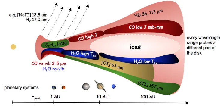
The interplay between critical density and excitation temperature in defining the optimum emit-ting conditions for various types of transitions and molecules is shown in figure 1 in the chapter by Dionatos (2015). It nicely illustrates that the various types of CO lines ranging from low rotational
9thLecture of the Summer School “Protoplanetary Disks: Theory and Modelling Meet Observations” DOI: 10.1051/
C
Owned by the authors, published by EDP Sciences, 2015 /201
epjconf 51020 0 1 00
lines to high rotational lines and then ro-vibrational transitions have the potential to probe the entire disk from the low density cold outer regions to the very hot, dense inner regions (see Fig. 1).
Figure 1.Disk sketch with the various molecular and atomic line emitting regions.
2 Statistical Equilibrium
Line fluxes depend on the level populations, or more directly on the column density of an atom/molecule in the upper energy level. We will simplify the radiative transfer for a moment and only consider the probability,β, that a line photon, emitted somewhere in a column of gas that we study, escapes the medium. The escape probability depends on the optical depthτul at line center frequencyνul. We will explain that concept later in more detail (see also chapter by Woitke 2015) and also get back to the full radiative transfer. Then, we can write the relation between the column density of the upper level,Nu, and the line fluxFulas
Ful≈NuAulhνulβ(τul)Ωsource
4π , (2)
whereAulis the Einstein coefficient for spontaneous emission andΩsourcethe solid angle of the line emitting region. This equation directly illustrates the importance of determining the level populations to calculate the column densities and hence compute line fluxes. In the following, we will discuss how to calculate these level populations in LTE and non-LTE (statistical equilibrium, SE).
2.1 Local Thermodynamic Equilibrium
In the case of LTE, the level populations within a specific ionization state of an atom or molecule are given by the Boltzmann equation
nu nl =
gu
gl
wherenu andnl are the level populations of the upper and lower energy level and gu andgl their statistical weights, respectively. ΔE=Eu−Elis the energy difference between the two levels,kthe Boltzmann constant andT is the gas temperature. Note that even if LTE does not hold, one can still define an excitation temperatureTexthat relates the two level populations through
nu nl =
gu
gl
e−ΔE/kTex. (4)
2.2 Ionization Equilibrium
The ionization balance of atoms and molecules in LTE follows from the Saha equation
n(Xi+1) n(Xi) =
(2πmkT)3/2 h3n
e
2Z(Xi+1) Z(Xi)
exp
−χi,i+1 kT
, (5)
wheren(Xi) is the level population in the ionization stateXiof the atom/molecule,neis the electron density,χi,i+1is the ionization energy from stateXitoXi+1,mis the mass of the atom/molecule, and Tis the gas temperature. The partition functionZ(Xi) of the ionization stateXiis defined as
Z(Xi)=
j
gje−Ej/kT . (6)
2.3 Non Local Thermodynamic Equilibrium
If the assumption of LTE breaks down, we have to solve the equations for non-LTE statistical equi-librium (SE). This means that we need to take into account all radiative and collisional processes that govern the distribution of level populations. The radiative processes are subject to the quantum mechanical selection rules and comprise spontaneous emission, stimulated emission and absorption, which depend on the respective Einstein coefficients. Collisional coupling can occur between any two levels; however, collision cross sections are generally larger between closely spaced energy levels and dipole allowed transitions. For each energy level, we can balance the rate for processes populating that level and those de-populating that same level. In equilibrium,dn/dt=0 holds, wherenis the vector containing all level populationsni.
The complete set of equations for SE becomes then
dni
dt =
j>i nj
Aji+BjiP(νji)
+
j<i
njBjiP(νji)+
ji
njCji (7)
−ni
j<i
Ai j+Bi jP(νi j)
−ni
j>i
Bi jP(νi j)−ni
ji Ci j .
The first term sums over all emissions from higher levels ending up in leveli, the second term over all absorptions from lower levels into leveli. The third term adds up all collisional ratesCjifrom lower and higher levels into leveli. The fourth to sixth term add up the respective radiative and collisional depopulation of leveli. P(νi j) denotes the local mean intensity averaged over ray directionsn and local line profile functionsφi j(ν, n) as
P(νi j)= 1
which can cause absorption and stimulated emission. Iν(n) is the spectral intensity at frequencyνin directionn. The three different Einstein coefficients for spontaneous emissionAji, stimulated emission Bji, and absorptionBi jare coupled through the following relations
Bji= c2
2hν3Aji (9)
and
giBi j=gjBji. (10)
Note that the exact form of these relations (first term of constants) depends on the units in which the radiation field is given.
This set of equations can be written in vector form as
Mn=b, (11)
wherenis an N-dimensional vector composed of the individual level populationsnifor all N levels andMis anN×Nmatrix composed of elementsMi j. For example, the columnuwithu>icontains the elements
Miu=(Aui+BuiP(νui)+Cui) . (12)
The largest amount of work lies in the compilation of all the atomic/molecular data, i.e. the level energies, statistical weights, radiative transitions, Einstein A coefficients, collision cross sections. Several databases provide this data such as the LAMDA database (Schöier et al. 2005), NIST, and CHIANTI (Dere et al. 1997).
2.4 Solving the Statistical Equilibrium
Once all radiative and collisional data is compiled for a specific atom/molecule, Eq. (11) can be inverted and solved forn. We need to respect, however, a very important boundary condition, namely the particle conservation that ensures that the sum of all level populationsniadds up to the total density of that atom/moleculentot. The way to impose this implicitly in the solution of the SE equation is to replace one of the equations in Eq. (11) with the conservation equation
i
ni=ntot. (13)
The matrixMthen becomes
M= ⎡ ⎢⎢⎢⎢⎢ ⎢⎢⎢⎢⎢ ⎢⎢⎢⎢⎢ ⎢⎢⎢⎢⎢ ⎣
M11 M12 · · · M1N−1 M1N M21 M22 · · · M2N−1 M2N
..
. ... ... ... ...
MN−11 MN−12 · · · MN−1N−1 MN−1N
1 1 · · · 1 1
⎤ ⎥⎥⎥⎥⎥ ⎥⎥⎥⎥⎥ ⎥⎥⎥⎥⎥ ⎥⎥⎥⎥⎥ ⎦ b= ⎡ ⎢⎢⎢⎢⎢ ⎢⎢⎢⎢⎢ ⎢⎢⎢⎢⎢ ⎢⎢⎢⎢⎢ ⎣ 0 0 .. . 0 ntot ⎤ ⎥⎥⎥⎥⎥ ⎥⎥⎥⎥⎥ ⎥⎥⎥⎥⎥ ⎥⎥⎥⎥⎥ ⎦ . (14)
2.5 The Two-level Atom
To provide better insight into the SE, we will in the following consider the two-level atom as an example. The atom has two energy levels with populationsn0andn1, which are connected through a single line with frequencyν10that has an Einstein coefficientA10. The SE in Eq. (7) becomes in that case
dn1
dt =n0B01P(ν10)+n0C01−n1[A10+B10P(ν10)]−n1C10=0 (15)
We can re-arrange this equation to isolate the ratio between the two level populations — making also use of the relations between the EinsteinAandBcoefficient —
n1 n0 =
A10 c 2 2hν3
10 g1
g0P(ν10)+C01
A10+A10 c 2 2hν3
10
P(ν10)+C10
. (16)
We see immediately that in the absence of a radiation field,P(ν10)=0, this simplifies to
n1 n0 =
C01 A10+C10
. (17)
Using the relation between the upwards and downwards collision rates
C01 C10 =
g1 g0
exp
− E10 kTgas
(18)
we find for very large collision rates (C10A10) that this equation becomes the Boltzmann equation. Hence, in that case, the two level populations are in LTE according to the local gas temperatureTgas.
An example of a simple two level atom is the two fine structure levels of the ground state of ionized carbon: Lower level2P3/2 and upper level2P1/2. They are separated by an energyE10 of 92 K and the emission line has a wavelength of 157.7μm. Since the critical density of this line is very low, it is widely observed in the interstellar medium (ISM, e.g. Pineda et al. 2013).
A second case to be considered is a situation where the collision rates are much smaller than the radiative rates (C10→0 andC01→0). In that case, Eq. (16) becomes
n1 n0 =
g1 g0
c2 2hν3
10 P(ν10)
1+2hcν23 10
P(ν10)
. (19)
IfP(ν10) is a blackbody radiation field of temperatureTgas, this becomes
n1 n0
= g1 g0
c2 2hν3
10
2hν3 10
c2 ehν10/kT1gas−1
1+ c2 2hν3
10
2hν3 10
c2 ehν10/kT1gas−1
=g1 g0
exp
− E10 kTgas
(20)
3 Radiative Transfer
Now that we understand how the different rotational, vibrational and electronic levels of an atom/molecule are populated, we can address the second part of understanding line emission: how does radiation cross the medium to reach the observer. From the equations of SE it became already evi-dent that the background radiation field can pump level populations under certain conditions. Hence, the two problems of SE and radiative transfer are closely intertwined, making the combined problem very difficult to solve even numerically. We will come back to that later when we address simplifi-cations made in disk research. The next few paragraphs will first illustrate the basic theory of line emission/absorption and line broadening.
3.1 Line Emission Coefficient
The line emission coefficientνi j is related to the EinsteinAcoefficient, the level population of the upper levelniand the line profile functionφi j(ν)
i j
ν = hνi j
4πniAi jφi j(ν) . (21)
The line profile function describes how a line at central frequencyνi j is broadened due to the uncer-tainty principle, collisions, thermal and turbulent motions in the gas, see Sect. 3.3. The line can also be Doppler-shifted by systematic motions of the gas in the observers frame, which causes the line profile function to become direction dependentφi j=φi j(ν, n) which is, however, not considered in this section. The line profile itself is normalized to one, φi j(ν)dν=1, with the effect that the total line emission is smeared out over a certain frequency range symmetric around the rest frequency of the lineνi j. A useful characterization of a line profile — also in observations — is the Full Width Half Maximum (FWHM), which measures the width of the profile at half its peak value.
3.2 Line Absorption Coefficient
The line absorption coefficientαi jν has two components, stimulated emissionBi jand absorptionBji. In that case, the sign of the absorption coefficient immediately hints to the presence of laser/maser1 emission, which will be discussed at the end of this chapter. The line absorption coefficient can be expressed as
αi j
ν = hνi j
4π
njBji−niBi j
φi j(ν), (22)
whereni andnj are the upper and lower level populations respectively andφi j(ν) is again the line profile function.
3.3 Line Broadening
The total line profile is a convolution of profiles from various types of broadening mechanisms: natural broadening, collisional broadening, thermal and turbulent broadening. The first two are related to the lifetime of the upper level of the transition and lead to a Lorentzian profile, while the second two cause Doppler shifts of the frequency and hence produce Gaussian profiles. The convolution of a Lorentzian and a Gaussian profile is a Voigt profile.
1Laser stands for Light Amplification by Stimulated Emission of Radiation and maser for Microwave Amplification by
Figure 2.Sketch of natural broadening (left), collisional broadening (middle) and thermal broadening (right).
Natural Broadening
Natural broadening is caused by the uncertainty principle. The shorter the lifetime of a state, the larger the energy uncertainty of the state
ΔEΔt∼= h
2π, (23)
and the natural line width thus becomes
Δν∼ ΔE
h ∼
1
2πΔt . (24)
The width of the profile is related to the spontaneous de-excitation rate from leveliinto all other levels j,γ=jAi j(Fig. 2). With this, the Lorentzian line profile can be written as (indicesi,jomitted)
φi j(ν)=
γ/4π2 (ν−νi j)2+(γ/4π)2
. (25)
Collisional Broadening
Atoms and molecules in a gas collide frequently and this reduces the lifetime in the different energy levels (Fig. 2). The broadeningΔνis proportional to the collision frequencyνcoll. Hence, collisional broadening becomes more important at higher densities. The line profile from the combined effect of natural and collisional broadening is still a Lorentzian
φi j(ν)= Δ
νtot/4π2 (ν−νi j)2+(Δνtot/4π)2
, (26)
with the widthΔνtotbeing the sum of the two widths (γ+2νcoll).
In most astrophysical cases, natural broadening is negligible. Collisional broadening plays mostly a role at very high densities, such as the ones reached in stellar atmospheres1012 cm−3. This leaves thermal and turbulent broadening as the dominant mechanisms under ISM, molecular cloud and protoplanetary disk conditions.
Thermal Broadening
The thermal velocities of atoms and molecules show a random Gaussian 3D velocity distribution (Fig. 3), a Maxwell-Boltzmann distribution
fv=2πv2
m 2πkTgas
3 exp
− mv2
2kTgas
Here, fv denotes the probability of finding an atom/molecule with a velocity close tov. The other quantities are the mass of the atom/moleculemand the gas temperatureTgas. Due to these random velocities, the frequency of the lineνi jis shifted according to the projected radial velocity component
vrin the line of sight to an observer
ν=νi j
1+vr c
. (28)
The resulting Doppler frequency shift is
ΔνD=νi j
vr
c . (29)
The most probable velocity of an atom/molecule of massmin a gas of temperatureTgasis
vr=vtherm =
2kTgas
m . (30)
A particle with this velocity has an energy ofkTgas. A simple expression to remember is the most probable velocity of a hydrogen atom
vtherm(H)=1.3
Tgas 100 K
1/2
km/s. (31)
From this, one can easily scale for atoms/molecules of different mass or a gas of different temperature. The line profile resulting from thermal Doppler broadening is a Gaussian profile
φi j(ν)= 1
ΔνD√πexp
⎛ ⎜⎜⎜⎜⎜ ⎜⎜⎜⎝−
ν−νi j
2
(ΔνD)2
⎞ ⎟⎟⎟⎟⎟
⎟⎟⎟⎠, (32)
with the widthΔνD(Eq. 29).
Turbulent Broadening
In the presence of turbulent motionsvturb, the width of the profile becomes
ΔνD= νi j
c
2kTgas
m +v
2 turb
1/2
. (33)
The root mean square of the thermal and turbulent velocities is often denoted by the parameterb in studies of the Interstellar Medium (ISM). Typical turbulent velocities for disks are inferred to be below 1 km/s.
The Gaussian profile is normalized to one. Its peak value atνi jand FWHM can be calculated from the width
φi j(ν)= 1
ΔνD
√π , FWHM=2 (ln 2)1/2ΔνD≈1.665ΔνD. (34)
Voigt profiles
A Voigt (V) profile is the convolution of a Lorentzian (L, widthΔνtot) and a Gaussian (G, widthΔνD) profile
V(ν,ΔνD,Δνtot)=
∞
−∞G(ν
,Δν
Figure 3.Left panel: Velocity distribution for hydrogen atoms at two different gas temperatures. Shown in color are the most probable, average and root mean square velocity of the distribution. Right panel: Comparison of a Lorentzian, Gaussian and Voigt profile.
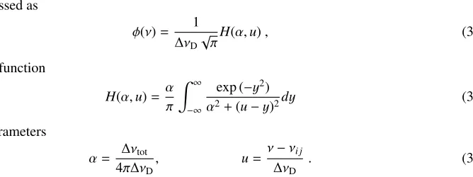
It can be expressed as
φ(ν)= 1
ΔνD
√πH(α,u), (36)
with the Voigt function
H(α,u)=α
π
∞
−∞
exp (−y2)
α2+(u−y)2dy (37)
and the two parameters
α= Δνtot 4πΔνD
, u=ν−νi j
ΔνD
. (38)
Fig. 3 (right panel) illustrates the shape of the Voigt profile in comparison with a Lorentzian and Gaussian, both having a FWHM of one and being normalized to one. The Voigt profile has wide damping wings (like the Lorentzian) and a Doppler core.
3.4 The Radiative Transfer Equation
The radiative transfer equation (RTE) describes how radiation is transported through a medium over a certain physical path lengths
dIν ds =α
ext
ν (Sν−Iν) . (39)
The absorption coefficient in units of cm−1is here the total extinction coefficient due to dust and line absorptionαext
ν =αdustν +αlineν φνwithφνbeing the line profile function. The source function is the ratio between the emission and absorption coefficients
Sν= dust
ν +νlineφν αdust
ν +αlineν φν
The dust emission coefficientνdustis composed of thermal emission and scattering, and can be calcu-lated from the dust temperatureTdustand the local mean intensityJν(assuming isotropic scattering)
dust
ν =αdustν ,absBν(Tdust)+αdustν ,scaJν, (41)
whereαdust
ν =αdustν ,abs+αdustν ,sca. Calculating these two quantities with continuum radiative transfer and various numerical methods, such as Monte Carlo, has been discussed in the chapter by Pinte (2015). Using the definition of optical depthdτν=−αextν ds, we can simplify the form of the RTE to
dIν
dτν =Iν−Sν. (42)
The formal solution of this equation can be written asJν(r) = Λν(r)Sν, whereΛν(r) is the famous Lambda integral operator. We can interpret this as a certain prescription operating on all source functions in the medium to obtain the frequency dependent radiation field Jν at positionr. If we imagine that we discretized our computational volume, the elements of theΛoperator couple each grid point with each other grid point in our volume. The coupling between SE and RT becomes evident in the source function, which contains the line emission and absorption coefficients, which in turn depend on the level populations (see Eq. 40).
3.5 Lambda Iteration
As stated above, the SE equations and the RTE are coupled. The source function depends on the radi-ation field itself, thus making the problem non-linear. Also, the level populradi-ations are local quantities and the radiation field is a global quantity. This means that local and global quantities are intrinsically coupled. Each iteration transports information roughly speaking over one mean free path of the pho-ton. This makes an iterative solution scheme very slow in propagating the local information through the medium. In the presence of large velocity gradients, many frequency points will be needed, again slowing down the computation. Last but not least, it has been shown that the pure Lambda Iteration converges even before the solution is reached and it does not necessarily converge to the true solution. Hence, defining convergence criteria is very hard.
The full problem can be solved by inverting theΛ operator. However, in the case of velocity gradients or broad line profiles, i.e. frequency coupling in a moving medium or across lines, the matrix can be very large. Hence, an iterative approach has numerical advantages over a straight inversion. Seminal references that describe the concept of the Lambda Iteration and the discretization are Mihalas (1978) and Kalkofen (1984). The basic scheme of the iteration procedure is outlined in Fig. 4 (left panel).
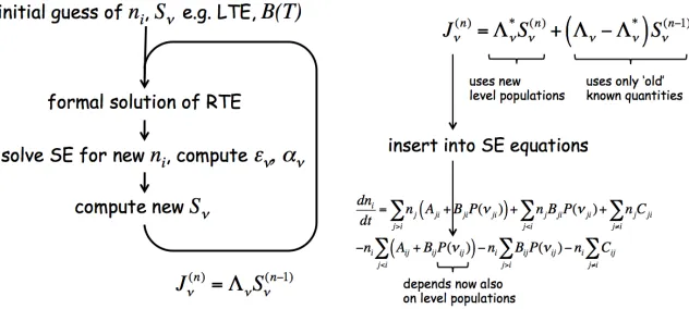
At the beginning of the iteration, LTE and a blackbody radiation field corresponding to the local temperature can be used as an initial guess for the level populationsni and the radiation field Jν allowing to compute the initial guess of the source functionS(0)ν . With this initial guess, the RTE can be formally solved for Jν(1). The radiation field is then used to solve the SE equations for the level populationsni. From these, the line absorption and emission coefficients can be calculated and also the new source functionS(1)ν . This leads to the iterative scheme
Jν(n)= ΛνS(νn−1). (43)
Figure 4.Left panel: Schematic flow of calculation for the Lambda Iteration (LI). Right panel: Improved concept of the Accelerated Lambda Iteration (ALI).
3.6 Accelerated Lambda Iteration
Having noted the convergence problems of the Lambda Iteration itself, we introduce now the more practical scheme of the Accelerated Lambda Iteration which in fact is much faster and does converge. Figure 4 (right panel) shows the basic idea of splitting the Lambda operator into two parts, an approx-imate Lambda operatorΛ∗ and the difference between the true and approximate Lambda operators (Λ−Λ∗)
J(νn) = Λ∗νSν(n)+Λν−Λ∗νS(νn−1). (44) This method presents an advantage if the approximate operator can be constructed in such a way that it is much simpler than the true operator but at the same time contains the essential properties of the true operator. Details on constructing such approximate operators can be found in the review by Hubeny (2003) and references therein. This method of an approximate Lambda operator is often called the method of deferred corrections (Cannon 1973). This becomes clearer, if we study the new scheme in detail: The approximate operator acts on the new source function, which depends on the new level populationsn(in). The second part of Eq. (44) makes only use old ’old’ known quantities. The solution of the RTE is then inserted into the SE equations. The radiation field enters in the absorption and stimulated emission terms. SinceJνnow depends onn(in), this makes the SE equations non-linear in theni’s and hence more difficult to solve. This is the price to pay at the end of the day.
3.6.1 Radiative Transfer in Disks
Because of the huge numerical efforts required to solve the coupled equations of SE and RT, the prob-lem is often approximately split between continuum and line radiative transfer. If the line emission has negligible effects on the overall radiation field, this approximation is not so bad. The SE equa-tions are then solved by using a simplified (sometimes multi-directional) escape probability approach, where the local radiation fieldP(νi j), which is used in the SE equations, is replaced by a mixture of the “background” continuum radiation fieldJcont
line “resonance” region, pumping the levels (Avrett & Hummer 1965). In 1D plane-parallel geometry, the intensity at the surfaceIνis related to the intensity at the bottomIν(0) through
Iν=Iν(0) e−τ+Bν(Texc)1−e−τ . (45)
Roughly speaking, e−τ gets replaced by the escape probability β(τ), where τ is the line optical depths along the considered ray direction. This approximation has problems if the geometry is multi-dimensional (no plane-parallel geometry) and the medium becomes optically thin. It will be discussed in more detail in the chapter by Woitke (2015). Finally, the line emission is calculated by performing ray tracing through the computational volume and using the level populations derived from the escape probability approach.
3.6.2 Velocity gradients
A protoplanetary disk has a Keplerian velocity field. This leads to double peaked velocity profiles as described in the seminal paper of Beckwith & Sargent (1993) and detailed in the chapter of Dionatos (2015). If a line photon is emitted in cellrn, it is shifted according to the Keplerian velocity of that cell. If the photon travels a distance s =rn−r(n−1) from one cell in the midplane to the next, this corresponds to a difference in velocitiesv(rn)−v(rn−1), and hence to a frequency shift of
Δνi j=νi j
v(rn)−v(rn−1)
c . (46)
If the frequency shift is larger than the line width, the photon is ’shifted out of the line’ and can escape. In Interstellar Medium physics, this is often referred to as the Large Velocity Gradient (LVG) approximation. It resembles the escape probability approximation discussed above since the escape probability can be written as
βesc=
1−e−τLVG
τLVG
, (47)
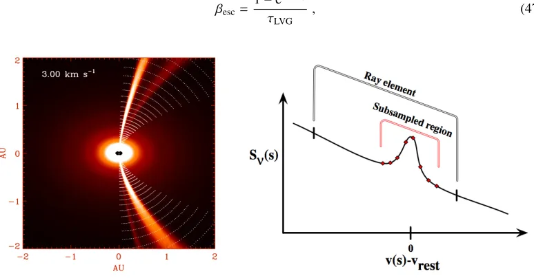
Figure 5.Left panel: Channel map of a line that is red-shifted by 3 km/s in a disk — visible are the front and back, but also the lower and upper disk part. Right panel: Sketch illustrating the concept of subsampling in the
case of large velocity gradients and a finite cell size. Figures from Pontoppidan et al. (2009, cAAS, reproduced
whereτLVG is the total optical depth along the path for any frequency. In disks, however, the LVG approximation does not work since a line photon can interact with the gas at various locations along a ray (e.g. top and bottom of the disk, near-side and far-side, Fig. 5, left panel). This problem is discussed in Pontoppidan et al. (2009) in detail for near-IR lines originating in the inner disk where velocity gradients across a cell can be large. In that case, the opacity needs to be properly sampled despite a finite cell size. To illustrate this, consider a typical turbulent/thermal broadening of<1 km/s and a grid with a resolution of 0.01 AU at a distance of 1 AU from the star. The velocity gradient across one cell is then∼4 km/s for a solar mass star. One possibility to ’catch’ the line within the cell is a subsampling of the source function between the cell boundaries (Fig. 5, right panel).
4 Special cases
After having discussed the foundations of the statistical equilibrium and radiative transfer, we will turn to a few special cases to illustrate the basic concepts.
4.1 Radiative pumping
The molecules in the disk surface are directly exposed to the stellar radiation field. This means that besides their statistical equilibrium being governed by the warm gas temperatures in the surface, ra-diative pumping can be very strong if the molecule has strong transitions in the UV/optical wavelength range, where the stellar radiation field peaks. An example is the CO molecule, which has electronic bands in the UV (4th positive system: A1Π−X1Σ+ around 1600 Å). Figure 6 illustrates the UV pumping of the upper electronic state and the cascade leading eventually to the emission of the CO ro-vibrational lines from the ground electronic state in the near-IR (∼4.6μm).
The stellar radiation field enters into the equations of SE through the absorption term
j<injBjiP(νji). The UV fluorescence can pump the populations in the upper vibrational levels of the ground electronic state to values much higher than LTE. Hence, the band ratios between the
v=1-0, 2-1, 3-2 bands will be affected and the hotter bands (v=2-1, 3-2) will get stronger with respect to the fundamental band (v=1-0). The mechanism counterbalancing this fluorescence is collisional
Figure 6. Left panel: Sketch of the CO fluorescence mechanism. Right panel: Sketch of the ortho- and para-water energy levels together with some key lines that have been observed with the Herschel satellite. Figures are
quenching (i.e. collisional de-population of the higherv-levels) due to high densities. The main colli-sion partner in the emitting region is atomic hydrogen (Thi et al. 2013) whose collicolli-sion rates are two orders of magnitude larger than those of molecular hydrogen.
Another example of radiative pumping is the water molecule. It has key transitions in the mid-IR where the spectral energy distribution of protoplanetary disks peaks. This means that the IR contin-uum photons (e.g. at 79 and 90μm) can efficiently pump low rotational levels of water. We saw in Sect. 2.1 that we can define an excitation temperatureTexfor any two levels. In the most extreme case of radiative pumping, the excitation temperature of the line would approach the local dust tempera-ture (optically thick case) or more precise the radiation temperatempera-ture of the continuum. This has been illustrated in the study of the water statistical equilibrium and radiative transfer in the disk around TW Hya (Kamp et al. 2013).
4.2 Masers
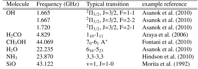
Maser (microwave amplification by the stimulated emission of radiation) emission is frequently ob-served in star forming regions and is often associated with massive star formation and Hiiregions. Maser emission is also seen in the vicinity of AGB stars. Table 1 gives an overview of detected maser transitions from molecules and references to the literature.
In order to observe a maser, we need an inversion of the level populations, so a collisional and/or radiative pumping mechanism. For the case of dusty environments around AGB stars, some possible pumping mechanisms for the 22 GHz water maser are described by Babkovskaia & Poutanen (2006). Characteristics of maser emission are large intensities, very narrow line width and unusual line ratios. The latter indicates very extreme non-LTE conditions. If multiple maser lines of the same molecule are observed from the same physical region, the excitation mechanism and the small scale structure and physical conditions in the gas can be disentangled.
Table 1.Examples of Maser transitions found in star forming environments and the vicinity of AGB stars.
Molecule Frequency (GHz) Typical transition example reference
OH 1.665 2Π
3/2, J=3/2, F=1-1 Asanok et al. (2010)
1.667 2Π
3/2, J=3/2, F=2-2 Asanok et al. (2010)
1.720 2Π
3/2, J=3/2, F=2-1 Asanok et al. (2010)
H2CO 4.829 110-111 Araya et al. (2006)
CH3OH 44.069 70-61A+ Fontani et al. (2010)
H2O 22.235 616-523 Asanok et al. (2010)
NH3 23.870 3,3-3,3 Hindson et al. (2010)
SiO 43.122 v=1, J=1-0 Morita et al. (1992)
4.3 Resonance scattering
Figure 7.Escape fraction of a Lyαphoton from a 1D slab model. Figure adapted from Neufeld (1990, cAAS, reproduced with permission).
Resonance scattering of Lyαphotons into the disk can increase the depth into the disk to which molecules can be photo dissociated. This occurs e.g. for molecules that have their dissociation bands overlapping with Lyαsuch as CO, OH, H2O and HCN (Fogel et al. 2011). Other molecules such as CN are unaffected. However, part of this can be compensated by an increased photodesorption rate also due to the enhanced Lyαradiation.
AcknowledgementsThe research leading to these results has received funding from the European
Union Seventh Framework Programme FP7-2011 under grant agreement no 284405. I would like to thank Irina Leonhardt and Odysseas Dionatos for a careful reading of the manuscript.
References
Araya, E., Hofner, P., Goss, W. M., et al. 2006, ApJL, 643, L33
Asanok, K., Etoka, S., Gray, M. D., et al. 2010, MNRAS, 404, 120
Avrett, E. H. & Hummer, D. G. 1965, MNRAS, 130, 295
Babkovskaia, N. & Poutanen, J. 2006, A&A, 447, 949
Beckwith, S. V. W. & Sargent, A. I. 1993, ApJ, 402, 280
Bergin, E., Calvet, N., D’Alessio, P., & Herczeg, G. J. 2003, ApJL, 591, L159
Cannon, C. J. 1973, JQRST, 13, 1011
Dionatos, O. 2015, in EPJ Web of Conferences, Vol. 102, Summer School on Protoplanetary Disks: Theory and Modeling Meet Observations, ed. I. Kamp, P. Woitke, & J. D. Ilee
Fogel, J. K. J., Bethell, T. J., Bergin, E. A., Calvet, N., & Semenov, D. 2011, ApJ, 726, 29
Fontani, F., Cesaroni, R., & Furuya, R. S. 2010, A&A, 517, A56
Hindson, L., Thompson, M. A., Urquhart, J. S., Clark, J. S., & Davies, B. 2010, MNRAS, 408, 1438
Hubeny, I. 2003, in Astronomical Society of the Pacific Conference Series, Vol. 288, Stellar Atmo-sphere Modeling, ed. I. Hubeny, D. Mihalas, & K. Werner, 17
Kalkofen, W., ed. 1984, Difference equations and linearization methods for radiative transfer (Auer, L. H.), 237–279
Kamp, I., Thi, W.-F., Meeus, G., et al. 2013, A&A, 559, A24
Mihalas, D. 1978, Stellar atmospheres/2nd edition/(San Francisco, W. H. Freeman and Co., 650 p.)
Morita, K.-I., Hasegawa, T., Ukita, N., Okumura, S. K., & Ishiguro, M. 1992, PASJ, 44, 373
Neufeld, D. A. 1990, ApJ, 350, 216
Pineda, J. L., Langer, W. D., Velusamy, T., & Goldsmith, P. F. 2013, A&A, 554, A103
Pinte, C. 2015, in EPJ Web of Conferences, Vol. 102, Summer School on Protoplanetary Disks: Theory and Modeling Meet Observations, ed. I. Kamp, P. Woitke, & J. D. Ilee
Pontoppidan, K. M., Meijerink, R., Dullemond, C. P., & Blake, G. A. 2009, ApJ, 704, 1482
Schöier, F. L., van der Tak, F. F. S., van Dishoeck, E. F., & Black, J. H. 2005, A&A, 432, 369
Stahler, S. & Palla, F. 2004, The Formation of Stars, Physics textbook (Wiley)
Thi, W. F., Kamp, I., Woitke, P., et al. 2013, A&A, 551, A49
van Dishoeck, E. F., Kristensen, L. E., Benz, A. O., et al. 2011, PASP, 123, 138