Regularized Integral Representations of the Reciprocal Function

Regularized Integral Representations of the

Reciprocal

Γ

Function

Dimiter Prodanov

Correspondence: Environment, Health and Safety, IMEC vzw, Kapeldreef 75, 3001 Leuven, Belgium; [email protected]; [email protected]

Version December 25, 2018 submitted to Preprints

Abstract:This paper establishes a real integral representation of the reciprocalΓfunction in terms 1

of a regularized hypersingular integral. The equivalence with the usual complex representation is 2

demonstrated. A regularized complex representation along the usual Hankel path is derived. 3

Keywords:gamma function; reciprocal gamma function; integral equation 4

MSC:33B15; 65D20, 30D10

5

1. Introduction 6

Applications of the Gamma function are ubiquitous in fractional calculus and the special function 7

theory. It has numerous interesting properties summarized in [1]. It is indispensable in the theory of 8

Laplace transforms. The history of the Gamma function is surveyed in [2]. In a previous note I have 9

investigated an approach to regularize derivatives at points, where the ordinary limit diverges [5]. 10

This paper exploits the same approach for the purposes of numerical computation of singular integrals, 11

such as the EulerΓintegrals for negative arguments. The paper also builds on an observations in [4]. 12

The present paper proves a real singular integral representation of the reciprocalΓfunction. The 13

algorithm is implemented in the Computer Algebra System Maxima for reference and demonstration 14

purposes. 15

As a second contribution, the paper provides an integral representation of the Gamma function for 16

negative numbers. Finally, the paper demonstrates an equivalent regularized complex representation 17

based on the regularization of the Heine integral. 18

2. Preliminaries and notation 19

The reciprocal Gamma function is an entire function. Starting from the Euler’s infinite product definition, the reciprocal Gamma function can be defined by the infinite product:

1

Γ(z) :=nlim→_∞

z(z+1). . .(z+n)

nz_n!

Proceeding from the Euler’s reflection formula for negative arguments the reciprocal Gamma function is simply

1

Γ(−z) =− sinπz

π Γ(z+1) (1)

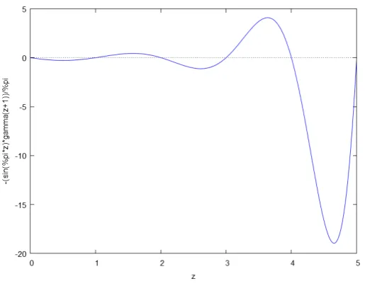
It is plot is presented in Fig.1. 20

Figure 1.1/Γ(−z)computed from Eq.1

The Euler’s Gamma function integral representation is valid for realz>0 or complex numbers, such thatRe z>0

Γ(z) =

Z ∞

0 e

−τ

τz−1dτ

however for negativezthe integral diverges. A less well-known integral representations forRe z<0 is the Cauchy–Saalschütz integral [6][Ch. 3]:

Γ(−z) =

Z ∞

0

e−τ_−e

n(−τ)

τz+1 dτ

The Hankel’s representation of the Gamma function is given as

Γ(z) = 1 2πisin(πz)

Z

Ha−e

τ

τz−1dτ, z6=0,−1,−2, . . .

The Heine’s complex representation for the reciprocal Gamma function is well known and is given below:

1

Γ(z) =

(−1)−z 2πi

Z

Ha+

e−τ

τz dτ=

1 2πi

Z

Ha− eτ

τz dτ

Here Ha− denotes the Hankel contour in the complexζ-plane with a cut along the negative real

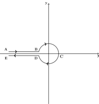
semi-axis argζ=πandHa+is its reflection. The contour is depicted in Fig.2. The integrand has a

simple pole atτ=0. The Hölder exponent at 0 can be computed in the closed interval[0,e]as

lim e→0

logee_e−z

loge =−z+lime→0

e

loge =−z

Therefore, fork>[z]it holds that lim e→0

ekeee−z=0 and the order of the residue is[z]. This observation 21

x y

C B

D A

E

Figure 2.The Hankel contourHa−.

2.1. Auxiliary notation 23

Definition 1. For a real number z the notation[z]will mean the integral part of the number, while{z}:= 24

z−[z]will denote the non-integral remaining part. 25

Definition 2. The falling factorial is defined as

(z)n := n−1

∏

z−k

Definition 3. Let

en(x):= n

∑

xk k!

be the truncated exponent polynomial sum under the convention e−1(x) =0. 26

3. Theoretical Results 27

Theorem 1(Real Reciprocal Gamma representation). Let z>0, z∈/Z and n= [z]. Then

1

Γ(z) = sinπz

π

Z ∞

0

e−x_−e

n−1(−x)

xz dx=Im

1

π

Z 0

−∞ ex_−e

n−1(x) xz dx where the integrals are over the real axis.

28

Proof. First, we establish two preliminary results. Consider the following limit of the form 0/0 and applyntimes l’Hôpital s’rule:

Lz= lim x→0

ex−en(x)

xz =

1 (z)nxlim→0

ex−1

xz−n Another application of l’Hôpital s’rule leads to

Lz= 1

(z)n(z−n)xlim→0e

Therefore,

Lz =



 

 

0, z<n+1

1

Γ(n+1), z=n+1

∞, z>n+1 Secondly, consider the limit

Mz = lim x→−∞

ex_−e n(x)

xz = Mz=_x→−lim_∞ ex xz −

n

∑

lim x→−∞

xk−z Γ(k+1)

Therefore,

Mz=



 

 

∞, z<n 1

Γ(n+1), z=n

0, z>n

Therefore, in order for both limits to vanish simultaneouslyn <z< n+1. Therefore,n = [z]. Let {z}=z−[z]. Then

In+1(z+1) =

Z 0

−_∞

ex−en(x) xz+1 dx=

ex−en(x) zxz ∞ 0 +1 z Z 0 −_∞

(ex−en(x))0 xz dx=

1

z

Z 0

−_∞

ex−en−1(x) xz dx=

1

zIn(z)

by the above results. Therefore, by reduction

In+1(z+1) = 1 (z)nI0

(z−n) = 1 (z)nI0

({z}) = 1 (z)n

Z 0

−∞ ex x{z}dx=

1 (z)n

Z ∞

0

e−x

(−x){z}dx=e

−iπ{z}Γ(1− {z}) (z)n Therefore,

Γ({z})In+1(z+1) = e

−iπ{z}

(z)n Γ(1

− {z})Γ({z}) =

e−iπ{z} π

(z)nsinπ{z} = π

(z)n(cot

π{z} −i)

by the Euler’s reflection formula. We take the imaginary part of the integral sinceΓ({z})is real and the middle expression is imaginary. Therefore,

1

Γ(z+1) = 1 (z)nΓ({z})

=Im1

πIn+1(z+1)

Finally,

1

Γ(z) =Im 1

π

Z 0

−∞

ex−en−1(x) xz dx 29

Corollary 1. By change of variables it holds that

1

Γ(z) = sinπz

πz

Z ∞

0 u

1

z−2 _e−u

1

z −

n−1

∑

(−1)kukz k!

!

du

Corollary 2(Modified Euler Integral of the second kind). By change of variables it holds that for z>0

1

Γ(z) = 1

π

Z 1

0

u−n∑−1 k=0

(logu)k

k!

u(logu)z du = sinπz

π

Z 1

0

1−en−1(logu)/u (log 1/u)z du

Finally, it is instructive to demonstrate the correspondence between the complex-analytical 31

representation and the hyper-singular representation. 32

Theorem 2(Regularized complex reciprocal Gamma representation). For z>0, z∈/Z and n= [z]

1

Γ(z) = 1 2πi

Z

Ha− eτ_−e

n−1(τ) τz dτ=

sinπz π

Z ∞

0

e−τ_−e

n−1(−τ) τz dτ whereτ∈R.

33

Proof. The proof technique follows [3]. We evaluate the line integral along the Hankel contour:

In(z) = 1 2πi

Z

Ha− eτ_−e

n−1(τ) τz dτ

with kernel

Ker(τ) = e

τ_−e

n−1(τ)

τz , z>0

The contour is depicted in Fig.2. The integral can be split in three parts

Z

HaKer

(τ)dτ=

Z

ABKer

(τ)dτ+

Z

BCDKer

(τ)dτ+

Z

DEKer (τ)dτ

along the rays AB, DE and the arch BCD, respectively. Along the ray AB whereτ =reiδthe kernel

becomes

KerA = 1

rz e eiδ_−iδzr

− n−1

∑

eiδk−iδz_rk k!

!

Along the ray DE whereξ=re−iδthe kernel becomes

KerB= 1 rz e

e−iδ_+iδzr −

n−1

∑

e−iδk+iδz_rk

k!

!

Therefore,

KerA−KerB= −2i

rz e

cos(δ)r _{sin(δz−sin(δ)r)−}

n−1

∑

cos(δk)rk k!

!

sin(δz) + n−1

∑

sin(δk)rk k!

!

cos(δz)

!

Therefore,

lim δ→π

1 2πi

Z 0

∞(KerA−KerB)dr=

sin(πz) π

Z ∞

0

e−z−en−1(−r)

rz dr

The integral on the arc BCD is given by the Cauchy Residue Theorem. By the above observation the residue atτ=0 is given by the limit

Res[Ker](τ) =lim

τ→0

τ1−z (eτ−en−1(τ)) = lim

τ→0

sinceLz=0. Therefore,

Z

BCDKer(τ)dτ=0 Furthermore, after integration by parts

In(z) =− e

τ_−e

n−1(τ)

τz−1

_Ha−

+ 1

2πi(z−1)

Z

Ha− eτ_−e

n−2(τ)

τz−1 dτ

= 1

z−1In−1(z) sinceMz=0. Therefore, the claim follows by reduction ton=0.

34

4. Applications 35

4.1. Laplace transform pairs 36

Consider the Laplace transformLs : f(t)÷F(s)As a concrete application of Th.2consider the pair

Ls :tk÷ Γ (k+1)

sk+1 , k>0 The inverse Laplace transform can be calculated simply as

L−_t1: Γ(k+1)

sk+1 ÷ 1 2πi

Z

Ha−Γ(k+1)

ets−e[k](ts)

sk+1 ds= sinπ(k+1)

πi Γ(k+1)

Z 0

−∞

ets−e_[k](ts)

sk+1 ds=t k

by change of variables. The latter result can be used for numerical inversion of Laplace transforms. 37

4.2. Ratios of Gamma functions 38

On a second place, the ratio of two Gamma functions can be represented as 39

Proposition 1. Let A,B>0. Then Γ(A)

Γ(B) = 1

π

Z 1

0

Z 1

0

1−en−1(logu)/u

(logu)B (−logv)

A−1_{du dv}

where n= [B]. 40

Proof.

Γ(A+1)

Γ(B) = 1

π

Z 1

0

1−en−1(logu)/u (logu)B du

Z 1

0 (−logv) A

dv= 1

π

Z 1

0

Z 1

0

1−en−1(logu)/u

(logu)B (−logv) A_{du dv}

41

4.3. The Cauchy–Saalschütz integral 42

Proposition 2. For z>0it holds that

Γ(−z) =−1

z

Z ∞

0

e−x−en−1(−x)

xz dx

Proof. By the reflection formula

Γ(1−z)Γ(z) = π

sinπz =−zΓ(−z)Γ(z)

Therefore,

Γ(−z) =− π

zsinπz

1

Γ(z) =− 1

z

Z ∞

0

e−x−en−1(−x)

xz dx

44

Remark 1. The latter result is equivalent to the classical Cauchy–Saalschütz integral representation. Indeed, by integration by parts

Γ(−z) =−1

z

Z ∞

0

e−x−en−1(−x)

xz dx=

1

z

Z ∞

0

d(e−x−en(−x))

xz =

e−x−en(−x) xz

∞

0

−−z

z

Z ∞

0

e−x−en(−x) xz+1 dx=

Z ∞

0

e−x−en(−x) xz+1 dx which is the Cauchy–Saalschütz integral.

45

5. Numerical Implementation 46

A reference implementation in the Computer Algebra System Maxima is given in Listings1and2. 47

The numerical integration code uses the library Quadpack, distributed with Maxima. The reference 48

implementation given in this section uses a routine for semi-infinite interval integration with tunable 49

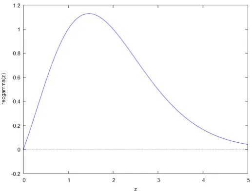
relative error of approximation (i.e. theepsrelparameter). A plot of the reciprocalΓfunction computed 50

from Listing1is presented in Fig.3. 51

Figure 3.1/Γ(z)computed from Th.1

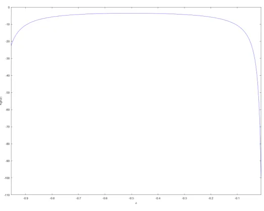
Figure 4.Γ(−z)computed from Prop.2

Listing 1: The Maixma code corresponsing to Th.1

1

53

Kg ( z ) : =b l o c k( [ u , r e t , k , n , f r : 1 , s s : 0 ] , 54

i f not numberp ( z ) then r e t u r n( ’ Kg ( z ) ) , 55

i f i n t e g e r p ( z ) then i f z=0 then r e t u r n( 0 ) e l s e r e t u r n( 1 / ( z−1 ) ! ) 56

e l s e ( 57

6 f r : s i n (% p i∗z)/%pi , 58

n : f i x ( z ) , 59

s s : sum ( (−u)^ k/k ! , k , 0 , n−1) , 60

r e t : f r∗f i r s t ( quad_qagi ( ( exp(−u)−s s )/ u^( z ) , u , 0 , i n f , ’ e p s r e l =1d−8)) 61

) , 62

11 f l o a t ( r e t ) 63

) ; 64

Listing 2: The Maixma code corresponsing to Corr.2

65

Kgn ( z ) : =b l o c k( [ u , r e t , k , n , f r : 1 , s s : 0 ] , 66

3 i f not numberp ( z ) then r e t u r n( ’ Kgn ( z ) ) , 67

i f i n t e g e r p ( z ) then r e t u r n( 0 ) 68

e l s e ( 69

i f z<0 then z:−z , 70

f r :−1/z , 71

8 n : f i x ( z ) , 72

s s : sum ( (−u)^ k/k ! , k , 0 , n−1) , 73

r e t : f r∗f i r s t ( quad_qagi ( ( exp(−u)−s s )/ u^( z ) , u , 0 , i n f , ’ e p s r e l =1d−8)) 74

) , 75

f l o a t ( r e t ) 76

13 ) ; 77

Acknowledgments: The work has been supported in part by a grants from Research Fund - Flanders (FWO), 78

contract number VS.097.16N and the COST Association Action CA16212 INDEPTH. Plots are prepared with the 79

computer algebra system Maxima. 80

References 81

1. J. M. Borwein and R. M. Corless. Gamma and factorial in the monthly.Am. Math. Monthly2018,125, 400–424. 82

2. P. J. Davis. Leonhard Euler’s integral: A historical pro 83

3. Y. Luchko. Algorithms for evaluation of the Wright function for the real arguments’ values.Fract. Calc. Appl. 85

Anal.2008,11, 57–75. 86

4. F. Mainardi.Fractional Calculus and Waves in Linear Viscoelasticity; Imperial College Press, 2010. 87

5. D. Prodanov. Regularization of derivatives on non-differentiable points.Journal of Physics: Conference Series 88

2016,701, 012031. 89