Evolve Then Filter Regularization for Stochastic
Reduced Order Modeling
Xuping Xie1,†*, Feng Bao2,‡and Clayton Webster3,† 1 Oak Ridge National Lab; [email protected]
2 Florida State University; [email protected] 3 Oak Ridge National Lab; [email protected]
* Correspondence: [email protected]
† Address: One Beth Valley Road, Oak Ridge National Lab, Oak Ridge, TN, 37831 ‡ Address: 1017 Academic Way, Tallahassee, FL 32306
1
2
3
4
5
6
7
8
Abstract: In this paper, we introduce the evolve-then-filter (EF) regularization method for reduced order modeling of convection-dominated stochastic systems. The standard Galerkin projection reduced order model (G-ROM) yield numerical oscillations in a convection-dominated regime. The evolve-then-filter reduced order model (EF-ROM) aims at the numerical stabilization of the standard G-ROM, which uses explicit ROM spatial filter to regularize various terms in the reduced order model (ROM). Our numerical results based on a stochastic Burgers equation with linear multiplicative noise. It shows that the EF-ROM is significantly better results than G-ROM.
Keywords: reduced order modeling; regularization; fluid dynamics; stochastic Burgers Equation; proper orthogonal decomposition; spatial filter
9
1. Introduction
10
Many important scientfic and engineering applications require repeated numerical simulations of
11
large and complex dynamical systems with high computational cost [25,26,40,45]. The traditional full
12
order model simulation is limited due to the extremely demanding on computational resources.
13
Reduced order models (ROMs), therefore, have been successfully introduced to reduce the
14
expensiveness of the numerical simulations. ROMs aim at finding a reduced space that approximate
15
the original model (full order model) with orders of magnitude reduction in computational cost
16
while maintaining high accuracy. The reduced space is constructed by truncating the reduced basis,
17
often the proper orthogonal decomposition (POD) basis. The classical Galerkin projection based
18
reduced order model (G-ROM) is one of the most popular model reduction method. It is obtained by
19
projecting the full order model to the reduced space. G-ROM is sucessful across a range of disciplines,
20
however, its’ use in convection-dominated flows has been hampered by the numerical instability. This
21
instability, usually in the form of unphysical numerical oscillations, yielding inaccurate results for
22
nonlinear systems. To mitigate the spurious numerical oscillations, various stabilized reduced order
23
models (ROMs) have been introduced see [2,5,13,24,31,32,42,44,54]. One popular strategy is theROM
24
closuremodeling which models the lost information in the truncation of the POD basis, many ROMs
25
can be found in [3,4,13,46,48,50,54,57]. Another approach is theregularization, which uses explicit
26
spatial filtering to regularize the standard G-ROM and increase the numerical stability of the ROM
27
approximation. Recent development of regularized ROMs method for deterministic systems have
28
been introduced in [47,55].
29
Reduced order models (ROMs) for systems involving stochastic process have gained increasing
30
attention recently [8,20,36]. The development of ROMs for partial differential equations (PDEs) subject
31
to random inputs acting on the boundary and PDEs with random coefficients have been considered
32
intensely in various contexts [16,27,53]. Some works have been done for ROMs for evolutionary PDEs
33
driven by stochastic processes [11,14]. [29] introduced the Leray-regularization reduced order model
34
(L-ROM) for the stochastic system with Brownian motions.
35
In this paper, we address the instability issue of standard G-ROM for nonlinear stochastic PDEs
36
by using regularization. Motiviated by [29], we introduce another regularized ROM, evolve-then-filter
37
(EF-ROM), for SPDEs that are of relevance to fluid dynamics as used in [29]. The main purpose is to
38
numerically investigate the evolve-then-filter regularization ROM (EF-ROM) for the stabilization of
39
the G-ROM within a simple setting, a stochastic Burgers equation (SBE) driven by linear multiplicative
40
noise. In [29], it has been shown that the spurious oscillations in G-ROM persist as the noise is turned
41
on, and the oscillations worsen as the noise amplitude increases. The numerical test of EF-ROM shows
42
that it gives more accurate modeling of the SBE dynamics by reducing the oscillations of the G-ROM
43
with a low dimensional approximation.
44
The rest of the paper is organized as follows. In Section2, we briefly describe the SBE to be used in
45
our numerical experiment. In Section3, we provide details about the derivation of the corresponding
46
G-ROM and EF-ROM based on proper orthogonal decomposition. In Section5, we present our
47
numerical investigation of the EF-ROM. Finally, we outline conclusions and potential future research
48
directions in Sectioin 6
49
2. Stochastic Burgers equation (SBE)
50
The deterministic viscous Burgers equation and its stochastic version have been widely used in reduced order modeling, see [14,15,34,39,49]. In this paper, we will focus on the following stochastic Burgers equation (SBE) driven by linear multiplicative noise:
du= νuxx−uuxdt+σu◦dWt,
u(0,t) =u(1,t) =0, t≥0, u(x, 0) =u0(x), x∈(0, 1),
(1)
whereu0is some appropriate initial datum to be specified,Wtis a two-sided one-dimensional Wiener
51
process,σis a positive constant that measures the “amplitude" of the noise, andνis a positive diffusion
52
coefficient. Similar to [29], the multiplicative noise term σu◦dWt is understood in the sense of
53
Stratonovich [41].
54
SPDEs driven by linear multiplicative noise such as the SBE (1) arise in various contexts,
55
including turbulence theory, non-equilibrium phase transitions, or simply the modeling of parameter
56
disturbance [6,12,18,38].
57
2.1. Numerical Discretization of SBE
58
In our numerical experiment at Section5, we collect the snapshots data from the direct numerical
59
simulation of the SBE. The SBE (1) is solved by a semi-implicit Euler scheme as given in [14, Section 6.1].
60
We briefly present the numerical discretization scheme below. For more details and other numerical
61
approximation methods of nonlinear SPDEs, see [1,7,11,28,30,37].
62
The nonlinearityuux= (u2)x/2 and the noise termσu◦ dWtare discretized explicitly for each
63
time step, while the other terms are treated implicitly. The Laplacian operator is discretized using the
64
standard second-order central difference approximation. Thus, we can get the following semi-implicit
65
discretization scheme:
66
uni+1−uni =ν∆uni+1+σ
2
2 u n i −
1 2∇(u
n i)2
∆t+σζnuni
√
∆t, (2)
whereun
i is the discrete approximation ofu(i∆x,n∆t),∆xand∆tare the mesh size of the spatial discretization and the time step, respectively. The discretized Laplacian∆and the discretized spatial derivative∇in (2) are given by
∆un i =
uni−1−2uni +uin+1
(∆x)2 ; ∇(u n i)2=
(uni+1)2−(uni)2
where the boundary conditions areun0 =unNx−1=0,Nxis the total number of grid points of the spatial
67
discretization in[0, 1]. Theζnare random variables drawn independently from a normal distribution
68
N(0, 1). The additional drift termσ2unj/2 in (2) is the conversion of the Stratonovich noise term
69
σu◦dWtinto Itô form.
70
2.2. Initial Condition
71
The initial condition is defined as following
u0(x) =
Z ∞
−∞ξ(y)φe(x−y)dy, x∈[0, 1]. (3) Whereξis the step function defined byξ(x) =1 ifx∈(0.05, 0.55)andξ(x) =0 otherwise. Theφeis given byφe(x) = 1eφ(xe)with
φ(x) =
Cexp − 1
(1−x2)
if|x|<1,
0 otherwise,
and the normalization constantCis chosen such thatR1
−1φ(x)dx=0. The parametereinφeis set to
72
bee=0.01 in our numerical experiment.
73
The initial condition is slightly modified from the one used in [34]. The modification is mainly
74
intended to enforce the compatibility of the initial and boundary condition at the left boundary point
75
(x=0) and to avoid any potential regularity issues that may arise in the numerical discretization of
76
the SBE in (2) due to the discontinuity in the step function.
77
3. Reduced Order Modeling
78
3.1. Proper Orthogonal Decomposition
79
POD is one of the most popular data-driven reduced order modeling method, which we
80
exclusively use to generate the ROM basis in this paper. We briefly describe the POD in this section.
81
We note, however, that other ROM bases (e.g., the dynamic mode decomposition (DMD)) could be
82
used. For more details, the reader is referred to [9,10,40,51]. The POD starts with the snapshots
83
{u0, . . . ,uNs}, which are numerical approximations of the SBE atNsdifferent time instances. The POD
84
seeks a low-dimensional spaceXr := span{ϕ1, . . . ,ϕr}that approximates the snapshots optimally
85
with respect toL2-norm.
86
Consider an ensemble of snapshotsR:=span
u0, . . . ,uNs , which is a collection of velocity data from either numerical simulation results or experimental observations at timeti =i∆t,i=0, . . . ,Ns. The POD basis{ϕ}icome from the minimization problem:
min 1
Ns+1 Ns
∑
`=0
u(·,t`)− r
∑
j=1
u(·,t`),ϕj(·)
ϕj(·)
2
(4)
subject to the conditions(ϕj,ϕi) =δij, 1≤i,j≤r, whereδijis the Kronecker delta. The minimization problem result in the eigenvalue problemKzj =λjzj, forj=1, . . . ,r, whereK∈R(Ns+1)×(Ns+1)is the snapshot correlation matrix with entriesKk` =
1
are given byϕj(·) = √1
λj ∑ Ns
`=0(zj)`uh(·,t`), 1 ≤ j ≤ r, where(zj)` is the`-th component of the eigenvectorzj. Also the following error formula holds from [26,34]:
1 Ns+1
Ns
∑
`=0
uh(·,t`)− r
∑
j=1
uh(·,t`),ϕj(·)
Hϕj(·) 2
= d
∑
j=r+1
λj. (5)
Note that in many ROMs of fluid dynamics, snapshots matrix always assembled by subtracting the
87
centering trajectory when generating the POD basis. That is, the fluctuationsu0=u−U, whereUis
88
the centering trajectory, are considered in the data matrix. For our numerical investigation, however,
89
we do not use the centering trajetory approach for the simple one dimension SBE case.
90
3.2. Galerkin Projection ROM (G-ROM)
91
The classic Galerkin projection based reduced order model has been introduced for fluids for many years. The derivation of the POD Galerkin ROM (G-ROM) follows the standard Galerkin approximation procedure. We present the derivation of G-ROM for the SBE (1) below. For a fixed number of basisr∼ O(10), ther-dimensional POD Galerkin approximationurof the SBE solutionu takes the following form:
ur(x,t;ω):=
r
∑
j=1
aj(t;ω)ϕj(x), (6)
where the time-varying coefficients (ROM coefficients){aj(t,ω)}rj=1are determined by solving:
dur,ϕj= ν(ur)xx−ur(ur)x,ϕjdt+σ ur,ϕj◦dWt, j=1,· · ·,r. (7)
Following the expansion ofurgiven in (6) and the orthogonality property of POD basis functions, we can get the more explicit form of the above equation:
daj=h−ν
r
∑
k=1
ak (ϕk)x,(ϕj)x+ r
∑
k,l=1
akal ϕk(ϕl)x,ϕj
i
dt+σaj◦dWt, (8)
where j = 1,· · ·,r. The above low dimensional dynamic system (8) is the called Galerkin ROM equation of the stochastic Burgers equation (SBE). The ROM online computation involves time integration of system (8), which carried out by using a standard Euler-Maruyanma scheme [33]. The fully discretized G-ROM of SBE is as follows:
anj+1−anj =h−ν
r
∑
k=1
ank (ϕk)x,(ϕj)x+ σ 2
2 a n j
+ r
∑
k,l=1
ankanl ϕk(ϕl)x,ϕj
i
∆t+σζnanj
√
∆t, j=1,· · ·,r,
(9)
whereζnare random variables drawn independently from a normal distributionN(0, 1).
92
4. Evolve-Then-Filter Regularized ROM
93
The G-ROM is efficient and relatively accurate for many fluid flows. As mentioned before,
94
however, G-ROM is inccurate for convection-dominated flows because of the numerical instability. In
95
this Section, we introduce and present details of the EF-ROM regularization for the SBE to investigate
96
potential improvement for numerical instability. This EF-ROM regularization based on POD spatial
97
filtering to smooth the flow variables and increase numerical stability of the model, see Sec.4.1.
4.1. POD Differential Filter
99
We present details of the ROM spatial filtering (Differential Filter) in this Section. ThePOD
100
differential filter (DF)is defined as follows: Letδbe the radius of the DF. For a givenur ∈ Xr, find
101
ur∈Xrsuch that
102
I−δ2∆
ur,ϕj
= (ur,ϕj), ∀j=1, . . .r. (10)
Differential filters have been used in the simulation of convection-dominated flows with standard
103
numerical methods [21,22]. The DF (10) uses anexplicit length scaleδ(i.e., the radius of the filter) to
104
eliminate the small scales (i.e., high frequencies) from the input. Indeed, the DF (10) uses an elliptic
105
operator to smooth the input variable. The DF also has a low computational overhead as it solves
106
a linear system with a very smallr×rmatrix that is precomputed. Another advantage is ROM DF
107
preserve incompressibility in the NSE, since they are linear operators. In reduced order modeling,
108
POD-DF was first used in [47] in a periodic, one-dimensional (1D) setting. In this paper, we apply
109
POD-DF to the SBE system (1).
110
4.2. EF-ROM for SBE
111
We draw inspiration from the deterministic case and considerregularized ROMs (Reg-ROMs)
112
constructed from the POD differential filter [55]. These Reg-ROMs belong to the wide class of stabilized
113
ROMs [2,3,5,13,17,24,32,42,46,54]. The main difference between Reg-ROMs and the other stabilized
114
ROMs is that Reg-ROMs increase the numerical stability of the model by usingexplicit spatial filtering,
115
which is a relatively new concept in the ROM field [47,54]. Other ROMs use closure modeling both
116
physically and mathematically. In this paper, we will use theEvolve-Then-Filter ROM (EF-ROM)[47,55]
117
based on a specific way of filtering the convective term in the SBE (1) as explained below.
118
The Evolve-Then-Filter model has been used as a numerical tool in the simulation of
119
convection-dominated deterministic flows with standard numerical methods [23,35]. It has also
120
been used to derive Reg-ROMs for deterministic systems in [47,55]. The construction of the EF-ROM
121
to the stochastic problem (1) is straightforward, which contains two steps. There is only one crucial
122
difference in its derivation compared to the derivation of the G-ROM as outlined in Section3.2, which
123
consists of applying POD-DF after evolving the dynamic system.
124
Ther-dimensional EF-ROM approximationur of the SBE solutionutakes the form (6). The
125
time-varying coefficients{aj(t,ω)}rj=1are determined by solving:
126
wrn+1−unr,ϕj
= ν(unr)xx−urn(unr)x,ϕjdt+σ unr,ϕj◦dWt, j=1,· · ·,r. (11)
unr+1 = wnr+1 (12)
The first "evolve" step in the EF-ROM (11) is just one step of the time discretization of the standard
127
G-ROM (9). The "filter" step in the EF-ROM consists of filtering of the intermediate solution obtained
128
in the "evolve" step:
129
I−δ2∆
wnr+1,ϕj
= (wnr+1,ϕj), ∀j=1, . . .r. (13)
wrn+1(t,x;ω)≡
r
∑
k=1
bk(t;ω)ϕk(x), (14)
This could give us the following linear system,
130
WhereMr= (ϕi,ϕj)andSr= (∇ϕi,∇ϕj)are the POD mass matrix and stiffness matrix respectively,
131
andbis the filtered POD coefficient. Thus ther-dimensional EF-ROM for SBE (1) is given by:
132
bnj+1−anj = h−ν
r
∑
k=1
ank (ϕk)x,(ϕj)x+ r
∑
k,l=1
ankanl ϕk(ϕl)x,ϕj
i
∆t+σζnanj ◦
√
∆t, (16)
anj+1 = bnj+1 (17)
wherej=1,· · ·,r. As mentioned in Section4, a forward Euler time discretization was used in (11),
133
but other time discretizations are possible [19].
134
Unlike the Leray-ROM (L-ROM) [29,58], which only filtering the nonlinear term, the EF-ROM
135
filter the whole dynamics of the coefficients after the "evolve" step. Some numerical analysis regard
136
these two methods for standard turbulent flows have been studied in [35]. A full comparison of the
137
Reg-ROMs for deterministic case was studied in [55]. We emphasize that a numerical comparison of
138
the EF-ROM and L-ROM for stochastic Burgers system is beyound the scope of this paper. A further
139
study with more discussions and complex stochastic systems will be investigated for future research.
140
5. Numerical Results
141
In this Section, we present our numerical results for the EF-ROM and compared it with the
142
standard G-ROM. The data that we used to construct our ROM is generated by the method describled
143
in Sec.2.1with the diffusion coefficientν=0.001,∆t=10−4andNx=1025 so that∆x ≈9.8×10⁻⁴.
144
We collected 101 equally spaced snapshots on the time interval[0, 1]and used method of snapshots
145
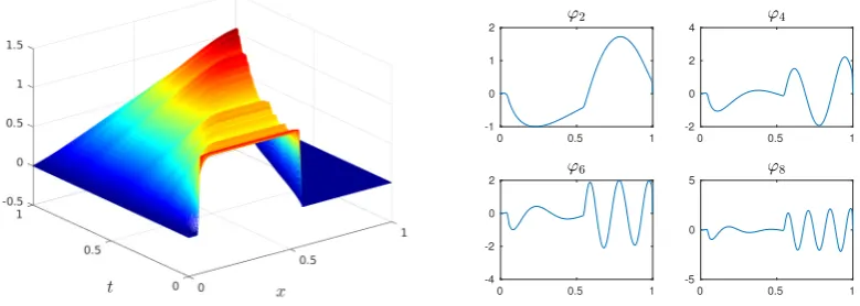
to compute the POD bases. The solution field and a few POD basis functions are shown in Fig.1for
146
illustration purposes.
0 0.5 1
-1 0 1 2
0 0.5 1
-2 0 2 4
0 0.5 1
-4 -2 0 2
0 0.5 1
-5 0 5
Figure 1.The numerical solution of SBE withσ=0.3 and the POD basis functions generated from the
solution data
147
Table 1.The energy captured by the first few POD basis from SBE data withσ=0.3.
No. of basis Energy
2 91.38%
4 97.20%
6 98.46%
8 99.02%
Even though the first few POD modes extract the most dominate percentage of energy, the
148
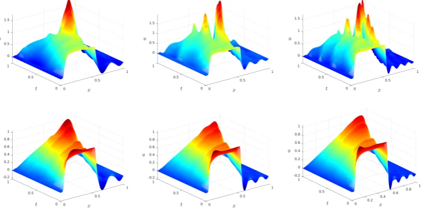
corresponding G-ROM generates a very high numerical oscillations, which yield inaccurate results.
This can be observed from the reconstructed ROM solution field in Fig.2. For the SBE problem studied
150
here, as we said before, the purpose of EF-ROM is to alleviate the spurious oscillations genearted
151
in standard G-ROM. We can see from Fig.2that, indeed, the oscillations are signifcantly reduced in
152
the spatio-temporal numerical reconstruction by EF-ROM resulting in a better approximation to the
153
original SBE system. Also note that as the dimension of the ROM increases, the overall performance of
154
both ROMs improves as can be seen in Fig.2. This behavior is expected since increasing dimensionr
155
increases the amount of energy used to the dynamic system of ROM, which accurately approximate
156
the SBE.
157
Figure 2.The space-time numerical reconstruction of SBE from G-ROM (9) (top row) and EF-ROM (16) (bot row) with dimensionr=4 (left panel),r=6 (middle panel) andr=8 (right panel), respectively. The noise path is the same as used in numerical solution of SBE field plotted in Fig.1
The parameterδthat defined as the radius of the ROM spatial filtering of EF-ROM in eqn. (13),
158
has to be appropriately calibrated to reach a good performance. Large value means filtering too much
159
of the spatial field which generate very bad results, while small value (identical to zero) means filtering
160
nothing just like the G-ROM. The optimal value (δ) is choosed by minimizing theL2-error of the
161
EF-ROM in numerical approximating the SBE’s spatio-temporal field. The noise (σ), dimensionrand
162
random variableζnin the numerical algorithm (16) can change the performance of the differentδ. To
163
reduce the numerical efforts, the nearly optimalδ=0.0011 is reached whenσ=0 forr=4, 6, 8, and
164
we fix thisδfor all the numerical (statistical) experiments.
165
Another comparison of the two ROMs can be made by looking the time evolution of the projected
166
coefficients onto each POD modes. The dynamics of POD coefficients can revel how the model perform
167
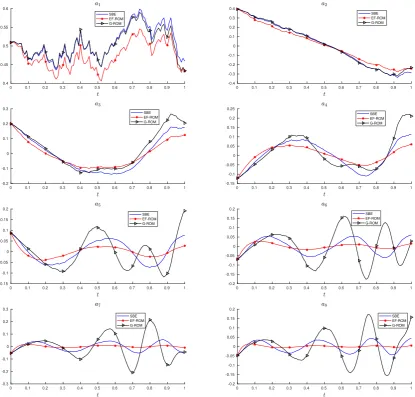
from the magnitude and the trajectory of each coefficient. Fig.3shows the evolution of POD coefficients
168
correspond to each POD basis. The two ROMs are perform quite well and similar for the leading
169
coefficientsa2anda3. For high frequency modes, however, G-ROM models badly about the dynamics
170
in terms of magnitude whereas EF-ROM generates a closer trajectory to SBE, see coefficientsa4−a8
171
in Fig.3. It is interesting to note that the EF-ROM leads a slight deterioration on the dynamic of first
172
modea1, see Fig.3. This deterioration is exist even if the optimalδis reached. The conjecutre is that the
173
DF spatial filtering affect this little deterioration. As the first POD mode contains the most dominant
174
energy, the filtering algorithm on the first mode would reduce its magnitude. The G-ROM, however,
175
uses exactly the same amount of energy which would approximate the first coefficient (a1) dynamic
better. Since this is our initial study, we intend to further investigate this issue together with more
177
complex stochastic systems and numerical analysis in our further research.
178
0 0.1 0.2 0.3 0.4 0.5 0.6 0.7 0.8 0.9 1 0.4
0.45 0.5 0.55 0.6
SBE EF-ROM G-ROM
0 0.1 0.2 0.3 0.4 0.5 0.6 0.7 0.8 0.9 1 -0.4
-0.3 -0.2 -0.1 0 0.1 0.2 0.3 0.4
SBE EF-ROM G-ROM
0 0.1 0.2 0.3 0.4 0.5 0.6 0.7 0.8 0.9 1 -0.2
-0.1 0 0.1 0.2 0.3
SBE EF-ROM G-ROM
0 0.1 0.2 0.3 0.4 0.5 0.6 0.7 0.8 0.9 1 -0.15
-0.1 -0.05 0 0.05 0.1 0.15 0.2 0.25
SBE EF-ROM G-ROM
0 0.1 0.2 0.3 0.4 0.5 0.6 0.7 0.8 0.9 1 -0.15
-0.1 -0.05 0 0.05 0.1 0.15 0.2
SBE EF-ROM G-ROM
0 0.1 0.2 0.3 0.4 0.5 0.6 0.7 0.8 0.9 1 -0.2
-0.15 -0.1 -0.05 0 0.05 0.1 0.15 0.2
SBE EF-ROM G-ROM
0 0.1 0.2 0.3 0.4 0.5 0.6 0.7 0.8 0.9 1 -0.3
-0.2 -0.1 0 0.1 0.2 0.3
SBE EF-ROM G-ROM
0 0.1 0.2 0.3 0.4 0.5 0.6 0.7 0.8 0.9 1 -0.2
-0.15 -0.1 -0.05 0 0.05 0.1 0.15 0.2
SBE EF-ROM G-ROM
Figure 3.Time evolution of the projected POD coefficients from the solution of G-ROM, EF-ROM and SBE system. The ROM solutions are obtained withσ=0.3 andr=8
Robustness of EF-ROM.
179
We also did numerical experiments regarding the statistical relevance of the ROM results.
180
Especially, we investigated the effect of the magintude of the noise on the results. The following
181
relativeL2error formula is used when assess the performance of the ROMs:
182
E(ω) =
q
R
|u(t;ω)−ur(t;ω)|2dX
q
R
|u(t;ω)|2dX
0.1 0.2 0.3 0.4 0.5 0.6 20
30 40 50 60 70
0.1 0.2 0.3 0.4 0.5 0.6
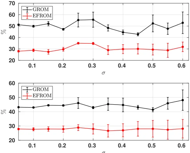
20 30 40 50 60
Figure 4.The ensemble averages of the relativeL2error of G-ROM (dark line) and EF-ROM (red line) computed via (18) for dimensionr=6 (top) andr=8 (bottom). The noise amplitudeσequally spaced
between 0 and 0.6. For eachσ, 1000 simulations are carried out for SBE and ROMs. The error bars show
the standard deviations.
For this experiment, we use 13 noise magnitudeσthat equally spaced between 0 and 0.6, and
183
perform 1000 simulations for each ROM. The related SBE solution data generated by the same size of
184
simulations via eqn. (2), and POD basis also updated at each simulation. The differential filter radius
185
δis fixed to be 0.0011. Fig.4plot the ensemble averages of the relative errors where the error bars
186
indicate the standard deviations. This result shows that the EF-ROM is significantly more accurate to
187
noise variations than G-ROM. The ensemble averages of error are above 40% for GROM withr=6
188
andr=8, while the EF-ROM relative error is around 30% (r=6) or below (r=8).
189
6. Conclusions
190
The numerical instability of Galerkin projection based ROMs is a very important challenge and
191
has been widely studied. We are investigating this challenge in the stochastic fluid flows background.
192
Motivated by few previous work [29], we introduced the evolve-then-filter (EF) regularized ROM for
193
stochastic fluids by performing a computational study of SBE. The EF-ROM uses the explicit spatial
194
filtering to regularize outputs from the ROM. The numerical results studied in this paper indicated
195
that the EF-ROM indeed alleviate the spurious oscillations that existed in the standard G-ROM. It
196
turned out that EF-ROM generates significant better approximation than G-ROM and less sensitive
197
to noise magnitude variaitons. We emphasize that although we use the same filtering method as in
198
regularized L-ROM [29], the model is fundamentally different. A comparison of EF-ROM and other
199
regularized ROMs (Reg-ROMs) is beyond the scope of this paper. We plan to have a thorough study of
200
Reg-ROMs for stochastic fluids in future research.
201
There are still many unclear questions need to be investigated. For example, does the EF-ROM
202
works for other different types of noise? e.g, addivie noise, correlated noise etc. How this ROM perform
203
for realistic 3D stochastic flows? Also how to propose new ROM method with the recently popular
204
data-driven ROM idea which applied machine learning or neural network inference [43,48,57,59]. It is
205
meaningful to research the robustness of the dynamics of ROM system with parameters (e.g,δ,ν,r,σ).
A good future direction would be provide a systematic approch corporate with machine learning to
207
predict the dynamics of ROM for stochastic system.
208
Author Contributions:Investigation, Xuping Xie; Methodology, Feng Bao; Project administration, Clayton G. 209
Webster; Writing – original draft, Xuping Xie; Writing – review & editing, Feng Bao and Clayton G. Webster. 210
Funding:This work is supported by the Scientific Discovery through Advanced Computing (SciDAC) program 211
funded by U.S. Department of Energy, Office of Science, Advanced Scientific Computing Research and Basic 212
Energy Sciences, Division of Materials Sciences and Engineering. The second author also acknowledges the 213
support from U.S. National Science Foundation under grant number DMS-1720222. 214
Acknowledgments:We would like to thank Prof. Traian Iliescu and Dr. Honghu Liu for the helpful suggestions. 215
Conflicts of Interest:The authors declare no conflict of interest. 216
Abbreviations
217
The following abbreviations are used in this manuscript: 218
219
ROM Reduced order modeling
EF-ROM Evolve then filter reduced order model G-ROM Galerkin reduced order model
POD Proper orthogonal decomposition
DF Differential filter
SBE Stochastic Burgers equation
220
221
1. Alabert, A.; Gyöngy, I. On numerical approximation of stochastic Burgers’ equation. InFrom Stochastic
222
Calculus to Mathematical Finance; Springer, Berlin, 2006; pp. 1–15. 223
2. Amsallem, D.; Farhat, C. Stabilization of projection-based reduced-order models. Int. J. Num. Meth. Eng.
224
2012,91, 358–377. 225
3. Balajewicz, M.J.; Dowell, E.H.; Noack, B.R. Low-dimensional modelling of high-Reynolds-number shear 226
flows incorporating constraints from the Navier–Stokes equation. J. Fluid Mech.2013,729, 285–308. 227
4. Ballarin, F.; Manzoni, A.; Quarteroni, A.; Rozza, G. Supremizer stabilization of POD–Galerkin 228
approximation of parametrized steady incompressible Navier–Stokes equations. Int. J. Numer. Meth.
229
Engng.2015,102, 1136–1161. 230
5. Barone, M.F.; Kalashnikova, I.; Segalman, D.J.; Thornquist, H.K. Stable Galerkin reduced order models for 231
linearized compressible flow. J. Comput. Phys.2009,228, 1932–1946. 232
6. Blömker, D. Amplitude Equations for Stochastic Partial Differential Equations; Vol. 3, Interdisciplinary
233
Mathematical Sciences, World Scientific Publishing Co. Pte. Ltd., Hackensack, NJ, 2007; pp. x+126. 234
7. Blömker, D.; Jentzen, A. Galerkin approximations for the stochastic Burgers equation. SIAM J. Numer.
235
Anal.2013,51, 694–715. 236
8. Boyaval, S.; Le Bris, C.; Lelièvre, T.; Maday, Y.; Nguyen, N.C.; Patera, A.T. Reduced basis techniques for 237
stochastic problems.Arch. Comput. methods Eng.2010,17, 435–454. 238
9. Brunton, S. L.; Proctor, J. L.; Kutz, J. N. Compressive sampling and dynamic mode decompositionarXiv
239
preprint arXiv:1312.5186,2013. 240
10. Brunton, S. L.; Proctor, J. L.; Kutz, J. N. Discovering governing equations from data by sparse identification 241
of nonlinear dynamical systemsProccedings of the National Academy of Science,2016
242
11. Burkardt, J.; Gunzburger, M.; Webster, C. Reduced order modeling of some nonlinear stochastic partial 243
differential equations. Inter. J. of Num. Anal. and Modeling2007,4, 368–391. 244
12. Birnir, B.The Kolmogorov-Obukhov Theory of Turbulence: A mathematical theory of turbulence; Springer Briefs in 245
Mathematics, Springer, New York, 2013. 246
13. Carlberg, K.; Farhat, C.; Cortial, J.; Amsallem, D. The GNAT method for nonlinear model reduction: 247
effective implementation and application to computational fluid dynamics and turbulent flows. J. Comput.
248
Phys.2013,242, 623–647. 249
14. Chekroun, M.D.; Liu, H.; Wang, S.Parameterizing Manifolds and Non-Markovian Reduced Equations: Stochastic
250
15. Chekroun, M.D.; Liu, H. Finite-horizon parameterizing manifolds, and applications to suboptimal control 252
of nonlinear parabolic PDEs. Acta Applicandae Mathematicae2015,135, 81–144. 253
16. Chen, P.; Quarteroni, A.; Rozza, G. A weighted reduced basis method for elliptic partial differential 254
equations with random input data.SIAM Journal on Numerical Analysis2013,51, 3163–3185. 255
17. Cordier, L.; Abou El Majd, B.; Favier, J. Calibration of POD reduced-order models using Tikhonov 256
regularization. Int. J. Num. Meth. Fluids2010,63, 269–296. 257
18. Cross, M.C.; Hohenberg, P.C. Pattern formation outside of equilibrium.Rev. Mod. Phys.1993,65, 851–1112. 258
19. Ervin, V.J.; Layton, W.J.; Neda, M. Numerical analysis of filter-based stabilization for evolution equations. 259
SIAM J. Numer. Anal.2012,50, 2307–2335. 260
20. Galbally, D.; Fidkowski, K.; Willcox, K.; Ghattas, O. Non-linear model reduction for uncertainty 261
quantification in large-scale inverse problems. Int. J. Numer. Meth. Engng.2010,81, 1581–1608. 262
21. Germano, M. Differential filters for the large eddy numerical simulation of turbulent flows. Phys. Fluids
263
1986,29, 1755–1757. 264
22. Germano, M. Differential filters of elliptic type.Phys. Fluids1986,29, 1757–1758. 265
23. Geurts, B.J.; Holm, D.D. Regularization modeling for large-eddy simulation. Phys. Fluids2003,15, L13–L16. 266
24. Giere, S.; Iliescu, T.; John, V.; Wells, D. SUPG Reduced Order Models for Convection-Dominated 267
Convection-Diffusion-Reaction Equations. Comput. Methods Appl. Mech. Engrg.2015,289, 454–474. 268
25. Hesthaven, J.S.; Rozza, G.; Stamm, B. Certified Reduced Basis Methods for Parametrized Partial Differential
269
Equations; Springer, 2015. 270
26. Holmes, P.; Lumley, J.L.; Berkooz, G. Turbulence, Coherent Structures, Dynamical Systems and Symmetry; 271
Cambridge, 1996. 272
27. Haasdonk, B.; Urban, K.; Wieland, B. Reduced Basis Methods for Parameterized Partial Differential 273
Equations with Stochastic Influences Using the Karhunen–Loéve Expansion. SIAM/ASA Journal on
274
Uncertainty Quantification2013,1, 79–105. 275
28. Hou, T.Y.; Luo, W.; Rozovskii, B.; Zhou, H.M. Wiener chaos expansions and numerical solutions of 276
randomly forced equations of fluid mechanics. J. Comput. Phys.2006,216, 687–706. 277
29. Iliescu, T.; Liu, H.; Xie, X. Regularized reduced order models for a stochastic Burgers equation. arXiv
278
preprint arXiv:1701.011552017. 279
30. Jentzen, A.; Kloeden, P.E.Taylor Approximations for Stochastic Partial Differential Equations; Vol. 83,CBMS-NSF
280
Regional Conference Series in Applied Mathematics, SIAM, Philadelphia, PA, 2011. 281
31. Kaiser, E.; Morzyski, M.; Daviller, G.; Kutz, J. N.; Brunton, B. W.; Brunton, S. L. Sparsity enabled cluster 282
reduced order models for controlJ. Comput. Phys.2018,352, 388–409. 283
32. Kalashnikova, I.; Barone, M.F. On the stability and convergence of a Galerkin reduced order model (ROM) 284
of compressible flow with solid wall and far-field boundary treatment. Int. J. Num. Meth. Eng. 2010, 285
83, 1345–1375. 286
33. Kloeden, P.E.; Platen, E. Numerical Solution of Stochastic Differential Equations; Vol. 23,Applications of
287
Mathematics, Springer-Verlag, Berlin, 1992; pp. xxxvi+632 pp. 288
34. Kunisch, K.; Volkwein, S. Galerkin proper orthogonal decomposition methods for parabolic problems. 289
Numer. Math.2001,90, 117–148. 290
35. Layton, W.J.; Rebholz, L.G.Approximate Deconvolution Models of Turbulence: Analysis, Phenomenology and
291
Numerical Analysis; Springer, 2012. 292
36. Lassila, T.; Manzoni, A.; Quarteroni, A.; Rozza, G. A reduced computational and geometrical framework 293
for inverse problems in hemodynamics. International journal for numerical methods in biomedical engineering
294
2013,29, 741–776. 295
37. Lord, G.J.; Rougemont, J. A numerical scheme for stochastic PDEs with Gevrey regularity.IMA J. Numer.
296
Anal.2004,24, 587–604. 297
38. Muñoz, M.A. Multiplicative noise in non-equilibrium phase transitions: A tutorial. InAdvances in Condensed
298
Matter and Statistical Physics; Nova Science Publishers, Inc., 2004; pp. 37–68. 299
39. Nguyen, N.; Rozza, G.; Patera, A.T. Reduced basis approximation and a posteriori error estimation for the 300
time-dependent viscous Burgers’ equation. Calcolo2009,46, 157–185. 301
40. Noack, B.R.; Morzynski, M.; Tadmor, G.Reduced-Order Modelling for Flow Control; Springer Verlag, 2011. 302
41. Øksendal, B.Stochastic Differential Equations: An Introduction with Applications, 6th ed.; Springer-Verlag, 303
42. Pacciarini, P.; Rozza, G. Stabilized reduced basis method for parametrized advection–diffusion PDEs. 305
Comput. Meth. Appl. Mech. Eng.2016,15, 142–161. 306
43. Peherstorfer, B.; Willcox, K. Data-driven operator inference for nonintrusive projection-based model 307
reductionComput. Meth. Appl. Mech. Eng.2016,306, 196–215. 308
44. Proctor, J. L.; Brunton, S. L.; Kutz, J. N.. Dynamic mode decomposition with controlSIAM J. Appl. Dyna.
309
Sys.2014,274, 1–18. 310
45. Quarteroni, A.; Manzoni, A.; Negri, F.Reduced Basis Methods for Partial Differential Equations: An Introduction; 311
Springer, 2015. 312
46. Quarteroni, A.; Rozza, G.; Manzoni, A. Certified reduced basis approximation for parametrized partial 313
differential equations and applications. J. Math. Ind.2011,1, 1–49. 314
47. Sabetghadam, F.; Jafarpour, A. α regularization of the POD-Galerkin dynamical systems of the
315
Kuramoto–Sivashinsky equation.Appl. Math. Comput.2012,218, 6012–6026. 316
48. San, O.; Maulik, R. Machine learning closure for model order reduction of thermal fluids. Appl. Math.
317
Model.2018,60, 681–710. 318
49. San, O.; Iliescu, T. Proper orthogonal decomposition closure models for fluid flows: Burgers equations 319
arXiv preprint arXiv:1308.32762013. 320
50. San, O.; Maulik, R. Neural network closure for nonlinear model order reduction. Adv. Comput. Math.2018, 321
1–34. 322
51. Schmid, P.J. Dynamic mode decomposition of numerical and experimental data. J. Fluid Mech. 2010, 323
656, 5–28. 324
52. Sirovich, L. Turbulence and the dynamics of coherent structures. Parts I–III. Quart. Appl. Math. 1987, 325
45, 561–590. 326
53. Torlo, D. Stabilized reduced basis method for transport PDEs with random inputs. Master thesis,Università 327
degli Studi di Trieste, Trieste, SISSA International School(unpublished)2016. 328
54. Wang, Z.; Akhtar, I.; Borggaard, J.; Iliescu, T. Proper orthogonal decomposition closure models for turbulent 329
flows: A numerical comparison.Comput. Meth. Appl. Mech. Eng.2012,237-240, 10–26. 330
55. Wells, D.; Wang, Z.; Xie, X.; Iliescu, T. An evolve-then-filter regularized reduced order model for 331
convection-dominated flows. International Journal for Numerical Methods in Fluids2017,84, 598–615. 332
56. Xiao, D.; Fang, F.; Buchan, A.G.; Pain, C.C.; Navon, I.M.; Du, J.; Hu, G. Non-linear model reduction for the 333
Navier–Stokes equations using residual DEIM method. J. Comput. Phys.2014,263, 1–18. 334
57. Xie, X.; Wells, D.; Wang, Z.; Iliescu, T. Approximate deconvolution reduced order modeling. Computer
335
Methods in Applied Mechanics and Engineering2017,313, 512–534. 336
58. Xie, X.; Wells, D.; Wang, Z.; Iliescu, T. Numerical analysis of the leray reduced order model. Journal of
337
Computational and Applied Mathematics2018,329, 12–29. 338
59. Xie, X.; Mohebujjaman, M.; Rebholz, L.; Iliescu, T. Data-driven filtered reduced order modeling of fluid 339