a
Corresponding author: [email protected]
Influence of the velocity vector base relocation to the center of mass of
the interrogation area on PIV accuracy
Jan Kouba1,a, Jan Novotný2and Jiří Nožička1 1
Czech Technical University in Prague, Faculty of Mechanical Engineering, Department of Fluid Dynamics and
Thermodynamics, Technická 4, Praha 6 – Dejvice, 166 07, Czech Republic
Abstract. This paper is aimed at modification of calculation algorithm used in data processing from PIV (Particle Image Velocimetry) method. The modification of standard Multi-step correlation algorithm is based on imaging the centre of mass of the interrogation area to define the initial point of the respective vector, instead of the geometrical centre. This paper describes the principle of initial point-vector assignment, the corresponding data processing methodology including the test track analysis. Both approaches are compared within the framework of accuracy in the conclusion. The accuracy test is performed using synthetic and real data.
1 Introduction
From the origin of the Particle Image Velocimetry Method (PIV), a significant development took place both in the field of instrumentation as well as in the field of data processing. Original optical correlators have been today replaced with high-performance workstations with professional software applications for velocity field evaluations. Within the period of more than 25 years from the PIV method origin, it has been widely developed and its current systems are capable of measuring of all three velocity components in several adjacent parallel planes at frequencies of more than 10 kHz [2][7]. During the above-mentioned period, the calculation algorithms were improved several times and, with their help, the PIV method has become the most used methods in the experimental research and development in the sphere of aerodynamics and fluid mechanics. [7]. In spite of the dramatic development in the sphere of data processing, the most popular algorithm for data processing at present is still the method known as the multi-step correlation algorithm. Against the new and more precise methods, this method is advantageous for its robustness, promptness and user friendliness, due to which even a start-up experimentalist may achieve good results at its default setting. If compared to newer algorithms, such as the methods based on the Interrogation Area (IA) deformation with hybrid algorithms combining PIV and PTV (Particle Tracking Velocimetry) [1] that try to compensate the adverse influence of the velocity gradient, the conventional algorithm of the multi-step correlation is based on a mere iterative scheme with shifting of IA with regard to the
measured dispacement in the previous iteration. It is therefore obvious that this calculation scheme very sensitive to the velocity gradient presence inside IA [7]. The presented paper deals with the influence of the velocity gradient on the PIV measurement accuracy and some possibilities how to reduce its adverse effect to the total measurement error. In this paper, the influence of the measured vector location inside IA is monitored with regard to the uneven distribution of particles inside IA and consequently to the total measurement accuracy. For the study of this influence, both synthetic as well as real data obtained from the Couette flow measurements in a test stand have been used.
2 Gradient inside IA
The magnitude of the gradient inside IA influences negatively, on a large scale, the total accuracy of the PIV method. The gradient presence inside IA reveals itself in two major effects. The first effect is called “in-plane loss of pairs”[7], while the other one is the correlation peak broadening.[8]
2.1 'In-plane loss of pairs' effect
The gradient presence inside IA causes unequal displacements of particle images inside IA, due to which paired particles are lost at the IA boundaries. The number of missing pairs is changing depending on the gradient value, particle count and their distribution inside IA, which negatively influences the accuracy of the evaluated shift. At small gradient values, it is possible to eliminate DOI: 10.1051/
C
Owned by the authors, published by EDP Sciences, 2014 , 0 20 57 (2014)
/2 01 67 epjconf EPJ Web of Conferences
this undesirable occurrence by using the calculation scheme called as the “Multi-Step Correlation“. However, at higher values, this technique is inadequate with a decrease in the signal/noise ratio in the resulting correlation plane, which consequently leads to a decrease in the accuracy of the PIV method measurements.
2.2 Correlation peak broadening
The correlation peak broadening is an effect occurring only with the gradient presence. The broadening occurs perpendicularly to the gradient. This occurrence has been described in detail by Westerweel [8]. In its paper, he showed the variation of the displacement a, which can be defined according to Figure 1. to relation (1).
Figure 1. Scheme for the variation of the displacement derivation. On the left side, the field of particle image displacements in IA (in the middle) is shown
=∙ ´ (1)
The variation of displacement a is reliant on the gradient of particle images displacement
and on L´,which is a distance between the marginal particle images within the IA.The correlation peak broadening is then shown in Figure 2., which compares the cross-sections of the correlation planes.
Figure 2. A comparison of two cross-sections of correlation peaks (gray – original condition, without any gradient, black – correlation plane with a gradient)
The value of the variation in pixels should correspond to the width of the evaluated correlation peak in the direction perpendicular to the gradient. No deformation
image and particle sizes, their count inside IA, this value is changing) undesirable peak “splitting” will occur.
2.3 Correlation peak splitting
The necessary condition for the peak splitting (2) is that the value of the variation of displacement a must be higher than the particle image diameterdpi.
> (2) However, even if this condition is met, no peak splitting may occur, if the particles are distributed uniformly in the levels of the same displacements and elementary variation among them are less than dpi. This applies to the same particle images of the same intensity. If particles of various intensities are present, then this property will affect the correlation peak and its splitting may happen. A comparison of the distribution of particles of the same intensity and size is shown in Figure 3. and Figure 4. On the left side it can bee seen the distribution of the first IA image of particles, while on the right side is the cross-section of the calculated correlation peak.
Figure 3. A cross-section through the correlation peak (right) calculated from IA with an unequal distribution of particles z IA (left)
Figure 4. A cross-section through the correlation peak (right) calculated from IA with an additional particle image in order to get the particles distributed evenly in the displacement levels
2.4. Influence of the gradient to the accuracy
decreased; the fact that this broadening is different for each IA means that the RMS value grows. Another growth in the RMS values can be seen in the gradient value that causes the peak splitting. As the shape of the correlation peak depends on all particle images inside IA regardless of their respective positions in the dispacement levels and their intensities. Therefore, from the limiting value, when the condition (2) is met, the RMS value may equal to dpior higher.
3 Solution proposal
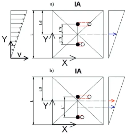
The evaluation of the measured dispacement by the use of the conventional multi-step correlation with the forward difference scheme will place the initial point of the evaluated displacement vector into the geometric centre of IA, which could be correct, if the particle were distribute uniformly and if they have the same intensity. However, it is practically impossible to achieve such an occurrence and therefore it is necessary to reflect that the initial point placed in this way is not, under the presence of the gradient inside IA, entirely correct. This is obvious from the next figure. Figure 5. shows in its section (a) a symmetrical distribution of particles and distance of the extreme particle images L´, the centre of which is in the IA geometric centre. Against this, the section (b) more realistic distribution of two particles, where the centre L´ is not at the geometric centre and the calculated average displacement of two particles is transferred into the IA geometric centre and to another displacement level.
Figure 5. A diagram of solution of an error occurring in the presence of the gradient inside IA
From the above consideration, the proposal of placing the evaluated displacement into the centre of mass of the IA [3].
4 Data processing methodology
For testing of the sensitivity of calculation algorithms, the synthetic Couette Flow Test was used. For a comparison with this regular test, data from the testing track with the Couette Flow have been used; they are described in the below paragraph.
The used synthetic data were generated with the background noise zero value, all particles had the identical diameter of 2.2 px, they did not overlap each other, they had approximately the same shape and intensity and they were distributed evenly along the whole IA. As the real data were burdened with lower or higher background noise and they contained particles of different sizes that are irregularly lighted due to their dissimilar positions inside the optical sheet, it was necessary to verify the synthetic test results in a real experiment.
The testing itself consists in comparisons of the results of the velocity profile known in advance with the velocity profile evaluated by use of PIV. The velocity profile for the Couette Flow derived from the basic equations of the fluid mechanics is a simple equation of straight line:
() = + (3)
The constant C1 represents the velocity gradient and C2
the velocity profile offset from the initial point of the system of coordinates. The case of flowing idealizedin this way is thus entirely suitable for testing of the accuracy of individual algorithms both in synthetic and real data. In the testing with the use of synthetic data, the whole process is very simple because the constants C1
and C2 are known in advance. In contrast to this, the
constant exact values in the Couette Flow measurements are influenced by a wide range of factors and burdened with a small error depending on the experiment execution accuracy. However, for the purposes of accuracy testing of individual algorithms, even this error is too large and the C1 and C2 constants had to be determined in another
way. From the given equation, the following criterion function can be constructed [4]:
(, ) = ∑ (− (+ ))
!
. (4)
The condition for the criterion function (4) prepared in this way is that its partial derivatives must be of zero value. Thus, for the criterion function two equations are in place necessary for obtaining of both constants, i.e. the constant represented the velocity gradient and the constant representing the offset of the velocity profile from the initial point of the system of coordinates. From the constants derived in this way, the theoretical velocity profile will be arranged again depending on the coordinates of the original vectors. The obtained
“theoretical” velocity profile will be consequently
deducted from the velocity profile evaluated by the PIV method. From the fluctuations remaining after the deduction of both velocity profiles, it is then possible to determine the so-called RMS error for the concrete velocity gradient.
5 Test track
The basis of the CFT test track consists of two rotating plates placed in a cylindrical vessel with the measuring liquid. The bottom plate is static, but the upper one performs a rotating motion. As the distance between these plates is adjustable, the height of the measuring space can be changed in the range from 5 to 50mm. The above-mentioned measuring space is in another square shape vessel with the liquid for better LASER sheet access and better visibility of the measuring area. The upper plate motions are provided by a machine assembly consisting of a worm-gear unit and an induction motor powered by a frequency convertor enabling the speed control.
A part of the test track is a frame with an attached optical path of lighting, which consists of a LASER diode with continuous lighting of 300mW and a couple of plano-convex cylindrical lenses. The first of the couple dilates the LASER beam to a plane so that the measuring space is uniformly lighted. The second lens provides for focusing into the measuring space so that the lighting sheet is in the place scanned by the camera as narrow as possible. The measuring track arrangement is shown in Figure 6.
Figure 6. Test track (1- measuring space, 2- camera, 3- LASER and optical path, 4- rotating plate drive)
Before the data measurement itself, it was necessary to prepare the track so that the acquired data would not show any undesirable noise and reflections from the neighbourhood and were thus as near as possible to the data used for synthetic tests. The data for the synthetic tests have zero values of the background noise, the signal is identical everywhere and the particle size is the same everywhere. For these reasons, fluorescent particles and the plates confining the measuring space were painted with the Mankiewicz NEXTEL® special coating to suppress undesirable reflections from the walls.
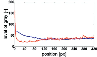
The comparison before and after the coating is shown in Figure 7. From the background signal course in the perpendicular direction to the wall (Figure 8.) it is evident the dramatic drop in the noise level at the wall after the application of the Mankiewicz NEXTEL® paint.
Figure 8. The background signal course for 8 bit resolution; blue – original condition, red – after the Mankiewicz NEXTEL® application
6 Experiment and acquired data
parameters.
Hamamatsu C9300-501 camera with the resolution of 1548x1548 px and Nikon AF Micro Nikkor 60mm objective lens, place on a camera stand and focused into the measuring space so that the image centre was also the rotation centre of the rotating plate, was used for the data recording. Fluorescent PMMA particles (diameter from 1 to 20μm) were used as the tracer particles [5]. Using a sugar solution, the water density was adjusted to the values corresponding to the particle density. Recordings and evaluations of acquired snapshots were carried out by the use of the Dynamic Studio 3.31 software application and the consequent assessment in the MATLAB program. Detailed experimental parameters are shown in the Table below.
Table 1. Experiment parametrs
Liquid density 1190±10 [kg•m-3]
Measuring space height 30 [mm]
Rotating plate revolutions 0.72 [rpm]
Frequency converter setting 10 [Hz] Measuring space distance from
the rotary centreline 56 [mm] Objective lens distance from
the measured area 150 [mm]
Exposure time 5000 [μs]
F-number 5.6 [-]
EFM 2013
The data acquired from the track adjusted in this way are shown in the Table below. The data are supported by the bar histograms – see Figure 9-12.These are the values of the highest frequency rate and only the added bar histogram completes the information about the acquired data quality.
Figure 9. Particle image diameter histogram for real measured data
Figure 10. Histogram for number of particles (IA 16x16)
Figure 11. Histogram for number of particles (IA 32x32)
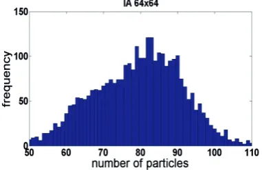
Figure 12. Histogram for number of particles (IA 64x64)
Table 2. Real measured data parameters
Background noise 4.8 %
Particle image diameter 3.6 px Number of particles IA 16x16 6 Number of particles IA 32x32 22 Number of particles IA 64x64 81
7. Results
As specified in Section 4, the testing has been carried out both with synthetic data and data acquired in real measurements. The synthetic data results (Figure 13.) may be considered for ideal results and their advantage consists in their simple analysis. However, it is necessary to take them with a slight reservation and complete them with the results from the data acquired in real measurements (Figure 14) that are more usable for practical use.
7.1. Synthetic data results
In the next chapter, the synthetic test results and their comparison with the conventional method without position corrections depending on the particle distribution inside IA are shown. Courses of percentile RMS deviations from the values reported for instance in [7],[6] are shown in the Figure 13. In the attached graphs, there is a noticeable trend of the RMS decrease to such gradient value that corresponds to the value level, from which the correlation peak splitting starts. This mainly obvious in the course for IA in the size of 64x64 px, where the peak-splitting limit corresponds to the gradient value of 0.034 px/px.
Figure 13. RMS reduction, synthetic data, no noise, dpi=2,2px
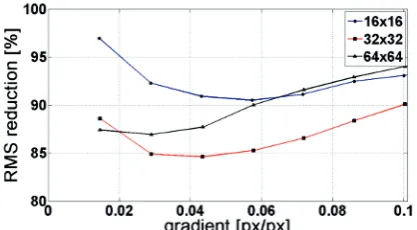
7.2. Results from the measured (real) data
Figure 14. RMS reduction for real measured data , dpi=2,2px,
background noise 4,8%
7. Conclusions
Based on the performed synthetic tests, a large potential has been verified for increased measurement accuracy at the position correction for the evaluated displacements as regards the uneven distribution of particles inside IA. It is obvious from the synthetic test results that by the correction the RMS error value can be decreased as low as to 40 % against the uncorrected value. Although the real test results confirmed the consistent trend in the RMS error value decrease, the final reduction was only at 85 to 90% against the original value. In the first place, the difference in the synthetic and real test results is given by the unequal sizes of particle images and their large scattering. New fluorescent particles with minimum scattering will have to be used for the synthetic test verifications. These particles were not available to us in the time of the experiment. After the new experiments are carried out, we assume that the synthetic test results will be confirmed.
8. Acknowledgement
This research has been realized using the support of Technological Agency, Czech Republic, programme Centres of Competence, project # TE01020020 Josef
Božek Competence Centre for Automotive Industry.
This support is gratefully acknowledged.
References
1. T. Astarita, G. Cardone, Exp. Fluids, 233-243, (2005)
2. H. Huang, D. Dabiri, M. GharibMeas. Sci. Technol. 8, 1427–1440, (1997)
3. R. Lindken, C. Poelma, J. Westerweel, Compensation for spatial effects for non-uniform seeding in PIV interrogation by signal relocation, Proc. 5th Int. Symposium on Particle Image Velocimetry (2003)
4. S. Miláček, Náhodné a chaotické jevy v mechanice,
5. J. Novotný, L. Manoch
,
Journal of MechanicsEngineering and Automation , 754-761,(2012) 6. J. Novotný, Journal of Flow Visualization and Image
Processing, 215-230, (2013)
7. M. Raffel, C. Willert, J. Kompenhans, Particle
Image Velocimetry : A Practical Guide, 2nd edition,
Berlin : Springer, (2007)