Volume 8, No. 3, March – April 2017
International Journal of Advanced Research in Computer Science RESEARCH PAPER
Available Online at www.ijarcs.info
Time Series Cross-Validation Techniques for determining the order of the
Autoregressive models
P.Kiran Kumar
Research Scholar, Department of Statistics Sri Venkateswara University Tirupati, Andhra Pradesh, India
Dr. B. Sarojamma
Assistant Professor, Department of Statistics Sri Venkateswara University Tirupati, Andhra Pradesh, India
Abstract: In the present research paper, we introduced some techniques of cross-validation for time series data. Six different types of time series cross-validation techniques are presented and also discussed various problems in selecting the initial training sample size and the size of training folds. In this paper, all cross-validation techniques, most appropriate techniques for model selection in time series analysis and advantages of the each technique are discussed with empirical study.
Keywords: Time series cross-validation, Prediction error, Order of AR model, Training sample, Test sample.
I. INTRODUCTION
Cross-validation is not only a method of choosing the best model but also a method of measuring accuracy. Since the order of the data is important in time series analysis, cross-validation might be problematic for time series models [1].
The application of cross validation to the time series data is not straight forward. The main reasons are
(i). Serial correlation in the data. (ii). Non-stationarity of the data.
The most appropriate cross-validation techniques are presented in the paper to determine the order of autoregressive model. These cross-validation techniques are useful for
a) Determining the order of autoregressive model and also the order of moving average model.
b) Selecting the best ARMA model among candidate models.
c) Selecting the best time series model among candidate models.
Consider the simple stationary linear autoregressive model of order ‘p’
1 1
t t p t p t
y =a y− ++a y− +ε
(
2)
whereεtare . .i i d N 0,σ
The number ‘p’ is called the order of the AR model. We need to choose ‘p’.
It can be written as yt =a x′ t+εt
Where a=
(
a a1, 2,,ap)
′ and xt =(
yt−1,yt−2,,yt p−)
′The autoregressive model of order ‘p’ fitted to the future data
{ }
1 m t t y = is
ˆ
t t t
y =a x′ +ε .
The process
{ }
yt mt=1 has the same distribution as the sampledata
{ }
yt tn=1but is independent of it, and(
1, 2, ,)
t t t t p
x = y− y− y− ′(Obviously, xtandxt do not
overlap) [2].
The prediction error measures the predictive ability of the estimated model by
{
}
2ˆ PE=E yt−a x′t
An estimate of PE using cross-validation is obtained on averaging the predictive square errors [3]. The following steps are used for estimate the predictive mean square error by cross-validation model selection procedures [4].
Step-1: Estimate a model based on a training sample.
Step-2: Forecast of a test sample is obtained by using the estimated model. It is denoted by ˆyα.
Step-3: Calculate the value of the predictive square error
(
)
2ˆ
yα −yα .
Hereyα is a set of observations of the test sample.
Step-4: Repeat Steps (1), (2) & (3) for each α and obtain
(
)
2ˆ PE=E yα −yα
The candidate models are
1: yt =a y1 t−1+εt
M
2:yt =a y1 t−1+a y2 t−2+εt
M
3: yt =a y1 t−1+a y2 t−2+a y3 t−3+εt
M
and so on
1 1 2 2 3 3
:
p yt =a yt− +a yt− +a yt− ++a yp t p− +εt
M
The best model or most appropriate autoregressive model of order O*for given a time series data is
* : t 1 t 1 2 t 2 3 t 3 * * t
O y =a y− +a y− +a y− ++a yO t O− +ε
M .
Where *
O ≤ p.
Shao(1993) defines the 'optimal model 'M O* , which
possess the smallest expected prediction error of any model
{
M O;O=1, 2, 3,p}
. Cross-validation estimates theexpected prediction error of a model and cross-validatory model selection proceeds by selecting the model with smallest estimated expected prediction error [5].
The optimal AR order *
O is chosen such that
( )
*{
( )
}
min O 1, 2, 3
TSCV O = TSCV O = p
Here TSCV O
( )
is the estimate of prediction mean squareerror in estimating the model M O [6].
Best model (i.e., optimal model) or most appropriate model
* O
II. TIME SERIES CROSS-VALIDATIONS TECHNIQUES
Six different types of cross-validation techniques introduced to determine the order of autoregressive process.
A. Time Series Cross Validation-1 Technique
[image:2.595.325.529.57.258.2]In time series cross validation-1 model selection procedure, there is a series of test samples; each test sample contains only one observation. The corresponding training samples consisting of the observations prior to the single observation of the test sample. It means that forecast at a time point is dependent on the past observations.
Figure 1. Time Series Cross Validation-1(TSCV-1)
In the figure-1,sample data
{ }
1 n t t
y = is repeatedly split into a
training sample (shown in grey colour) and a validation set (i.e., test sample) that contains only one observation (shown in black colour).
Training Samples:
{
y y1, 2yi k+ −1}
;i=1, 2,, n k−Test Samples:
{ }
yi k+ ;i=1, 2,, n k− (or){ }
1 nk yα α= +
Here k is minimum training sample size to estimate the model. An estimate of PE using TSCV-1 technique is
1
(
)
2ˆ
PE y y
n k α α
= −
−
∑
B. Time Series Cross Validation-2 Technique
In time series cross validation-2 model selection procedure, there is a series of test samples; each test sample contains only one observation. The corresponding training samples consisting of a number of observations prior to the single observation of the test sample. The TSCV-2 technique is similar to TSCV-1 technique, but the size of training sample in TSCV-2 technique is constant
.
Training Samples:
{
yi,,yi k+ −1}
;i=1, 2,, n k−Test Samples:
{ }
yi k+ ;i=1, 2,, n k− (or){ }
yα αn= +k 1Here k is minimum training sample size to estimate the model and is the size of training sample in each split.
An estimate of PE using TSCV-2 technique is
1
(
)
2ˆ
PE y y
n k α α
= −
[image:2.595.51.258.203.405.2]−
∑
Figure 2. Time Series Cross Validation-2(TSCV-2)
In the figure-2,sample data
{ }
yt tn=1 is repeatedly split into atraining sample (shown in grey colour), the size of the training samples are fixed and a validation set (i.e., test sample) that contains only one observation (shown in black colour).
C. Time Series Cross Validation-3 Technique
In time series cross validation-3 model selection procedure, there is a series of test samples; each test sample contains only one observation (i.e., 3-step-ahead data point). In time series analysis, multi-step forecasts are relevant than one-step forecasts. The TSCV-3 technique is a relevant selection procedure than TSCV-1 and TSCV-2 techniques.
Figure 3. Time Series Cross Validation-3(TSCV-3)
In the figure-3, sample data
{ }
yt tn=1 is repeatedly split into a training sample (shown in grey colour) and a validation set (i.e., test sample) that contains only one observation (shown in black colour). The single observation of the test sample is a 3-step-ahead data point.Training Samples:
{
y1,,yi k+ −1}
;i=1, 2,, n k 2− −Test Samples:
{
yi k+ +2}
;i=1, 2,, n k 2− − (or) [image:2.595.320.529.434.636.2]Here k is minimum training sample size to estimate the model. An estimate of PE using TSCV-3 technique is
1
(
)
2ˆ PE
2 y y
n k α α
= −
− −
∑
D. Time Series Cross Validation-4 Technique
In time series cross validation-4 model selection procedure, there is a series of test samples or test folds, each test fold contains a set of observations and test fold sizes are equal. The TSCV-4 technique is a good model selection procedure than TSCV-1, TSCV-2 and TSCV-3 techniques.
Assumption:
1. n is multiple of k
2. The size of first training fold is same as the size of first test fold.
3. Test folds are equal in size. It means that each test sample consists of an equal number of observations in it.
Figure 4. Time Series Cross Validation-4(TSCV-4)
Training Samples (or) Training folds:
{
1 2}
n k
, ;i 1, 2, ,
k
i k
y y y× = −
Test Samples (or) Test folds:
( ) ( )
{
1 1}
n k
, , ;i 1, 2, ,
k
i k i k
y × + y + × = −
Here k is minimum training sample size to estimate the model.
An estimate of PE using TSCV-4 technique is
( ) ( ) ( )
( )
2 3
2 2 2
1 2 1 1
1
ˆ ˆ ˆ
PE
+ + − +
= − + − + + −
−
∑
∑
∑
k k n
k k n k
y y y y y y
n k α α α α α α
Where
(
)
2 2 1 ˆ k kyα yα +
−
∑
is a total predictive square error of first testsample
{
yk+1,,y2k}
(
)
3 2 2 1 ˆ k kyα yα +
−
∑
is a total predictive square error of second testsample
{
y2k+1,,y3k}
(
)
( ) 2 1 ˆ n n kyα yα − +
−
∑
is a total predictive square error of last testsample
{
y(n k− +)1,,yn}
E. Time Series Cross Validation-5 Technique
In time series cross validation-5 model selection procedure, there is a series of test samples or test folds, each test fold contains a set of observations and test fold sizes are equal. The corresponding training samples consisting of the number of observations prior to the test sample. In TSCV-5 model selection procedure, the size of training samples and test samples are equal in each split.
Assumption:
1. n is multiple of k
2. The size of training fold is same as the size of test fold in each split.
[image:3.595.39.279.279.386.2]3. Test folds are equal in size. It means that each test sample consists of an equal number of observations in it.
Figure 5. Time Series Cross Validation-5(TSCV-5)
Training Samples (or) Training folds:
( )
{
1 1}
n k
, , ;i 1, 2, ,
k
i k i k
y+ − y×
− =
Test Samples (or) Test folds:
( ) ( )
{
1 1}
n k
, , ;i 1, 2, ,
k
i k i k
y × + y + × = −
Here k is minimum training sample size to estimate the model.
An estimate of PE using TSCV-5 technique is
( ) ( ) ( )
( )
2 3
2 2 2
1 2 1 1
1
ˆ ˆ ˆ
PE
+ + − +
= − + − + + −
−
∑
∑
∑
k k n
k k n k
y y y y y y
n k α α α α α α
Where
(
)
2 2 1 ˆ k kyα yα +
−
∑
is a total predictive square error of first test sample{
yk+1,,y2k}
(
)
3 2 2 1 ˆ k kyα yα +
−
∑
is a total predictive square error of second test sample{
y2k+1,,y3k}
(
)
( ) 2 1 ˆ n n kyα yα − +
−
∑
is a total predictive square error of last testsample
{
y(n k− +)1,,yn}
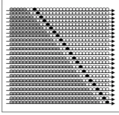
F. Time Series Cross Validation-6Technique
In time series cross validation-6 model selection procedure, there is a series of test samples or test folds, each test fold contains a set of observations which are k-step-ahead data points and test fold sizes are equal.
Assumption:
1. n is multiple of k
3. Test folds are equal in size. It means that each test sample consists of an equal number of observations in it.
Figure 6. Time Series Cross Validation-6(TSCV-6)
Training Samples (or) Training folds:
{
1}
n 2 k
, , ;i 1, 2, ,
k
i k
y y×
− =
Test Samples (or) Test folds:
( ) ( )
{
1 1 2}
n 2 k
, , ;i 1, 2, ,
k
i k i k
y + + y + = −
Here k is minimum training sample size to estimate the model.
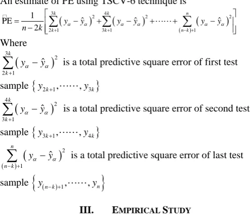
An estimate of PE using TSCV-6 technique is
( ) ( ) ( )
( )
3 4
2 2 2
2 1 3 1 1
1
ˆ ˆ ˆ
PE
2 + + − +
= − − + − + + −
∑
∑
∑
k k n
k k n k
y y y y y y
n k α α α α α α
Where
(
)
3
2
2 1
ˆ
k
k
yα yα +
−
∑
is a total predictive square error of first test sample{
y2k+1,,y3k}
(
)
4
2
3 1
ˆ
k
k
yα yα +
−
∑
is a total predictive square error of second test sample{
y3k+1,,y4k}
(
)
( )
2
1
ˆ
n
n k
yα yα − +
−
∑
is a total predictive square error of last testsample
{
y(n k− +)1,,yn}
III. EMPIRICAL STUDY
We generated a series of 250 observations from the autoregressive model of order 2,
1 2
0.58 0.65
t t t t
y = y− − y− +ε , whereεtare . .i i d N
( )
0,1 .The candidate models are
1:yt =a y1 t−1+εt
M
2:yt =a y1 t−1+a y2 t−2+εt
M
3: yt =a y1 t−1+a y2 t−2+a y3 t−3+εt
M
4:yt =a y1 t−1+a y2 t−2+a y3 t−3+a y4 t−4+εt
M
5: yt =a y1 t−1+a y2 t−2+a y3 t−3+a y4 t−4+a y5 t−5+εt
M
TSCV techniques are used to estimate the optimal order of autoregressive model.
The prediction mean square error for each candidate model is estimated by different TSCV techniques using R Software and these values are presented in table I to V.
Table I. Estimates of PE by TSCV-1 technique
k Estimates of PE by TSCV-1 technique for the Model
AR(1) AR(2) AR(3) AR(4) AR(5)
25 1.530311 0.973941 0.985433 1.014555 1.025889 50 1.582546 1.01608 1.02759 1.049468 1.059643 75 1.581222 1.00519 1.012122 1.034494 1.038942 100 1.423709 0.986364 0.992325 1.003767 1.007592 125 1.405905 0.993532 0.998706 1.012341 1.014716 150 1.33519 0.941361 0.946084 0.949703 0.951085 175 1.243363 0.934801 0.942493 0.94613 0.944047 200 1.595412 1.136492 1.145097 1.150882 1.146659 225 1.309337 0.770816 0.770429 0.769918 0.781212
For k=225, AR(4) model is the most appropriate model by TSCV-1 technique. Since the estimate of prediction error based on less number of observations, the TSCV-1 technique is not selecting the most appropriate model. The minimum number of observations required to estimate the prediction error is 40 in this situation. For remaining k values, TSCV-1 technique performs well.
Table II. Estimates of PE by TSCV-2 technique
In the TSCV-2 technique, the first observation in each training sample is not far from the observation of the test sample. A minimum number of observations in each training sample are not less than 10 % of the data is considered for the present study. For all selected values of k, TSCV-2 technique performing well.
Table III. Estimates of PE by TSCV-3 technique
k Estimates of PE by TSCV-3 technique for the Model
AR(1) AR(2) AR(3) AR(4) AR(5)
25 1.779215 1.371621 1.384179 1.399293 1.415454 50 1.835528 1.427255 1.436383 1.462076 1.474493 75 1.84689 1.438611 1.44419 1.471097 1.475356 100 1.63721 1.392555 1.395461 1.407555 1.408046 125 1.599433 1.334273 1.337071 1.349015 1.347026 150 1.451404 1.271021 1.272582 1.27731 1.274207 175 1.461919 1.237995 1.242911 1.251946 1.24351 200 1.647454 1.354596 1.35926 1.368044 1.354306
225 1.596424 1.185301 1.180439 1.176958 1.191044
The TSCV-3 technique is dependent on the observations of the test sample which is h-step ahead data point and the value of k. To select the most appropriate model, we chose h as 2, 3, 4 and 5. The TSCV-3 technique is performing well for the size of training sample which lies between 10% and 75% of the data. For the k (25 to 175) values, TSCV-3 technique performs well.
k Estimates of PE by TSCV-2 technique for the Model
AR(1) AR(2) AR(3) AR(4) AR(5)
[image:4.595.36.283.326.538.2] [image:4.595.302.567.549.684.2]Table IV. Estimates of PE by TSCV-4 technique
k Estimates of PE by TSCV-4 technique for the Model
AR(1) AR(2) AR(3) AR(4) AR(5)
5 1.491581 0.944388 0.958796 1.006564 1.014591 10 1.508478 0.970101 1.025693 1.021178 1.028944 25 1.514073 0.946957 0.951758 0.964936 0.971821 50 1.561074 1.012016 1.023154 1.056757 1.06298 125 1.406476 0.953078 0.953496 0.971115 0.970077
In the TSCV-4 technique, we chose the k value such that n k
k −
is an integer andk≥5. For all selected values of k,
TSCV-4 technique performs well.
For k=125, the training fold consisting of the first 50% of the data and the test fold consisting of the last 50% of the data.
Table V. Estimates of PE by TSCV-5 technique
k Estimates of PE by TSCV-5 technique for the Model
AR(1) AR(2) AR(3) AR(4) AR(5)
10 1.538369 1.02339 1.221861 1.19563 1.288271 25 1.522967 0.980885 0.995129 1.027841 1.134396 50 1.56086 1.010527 1.047324 1.071945 1.091911 125 1.406476 0.953078 0.953496 0.971115 0.970077
In the TSCV-5 technique, we chose the k value such that n k
k −
is an integer and k≥5. For all selected values of k,
TSCV-5 technique performing well.
For k=125, the training fold consisting of the first 50% of the data and the test fold consisting of the last 50% of the data.
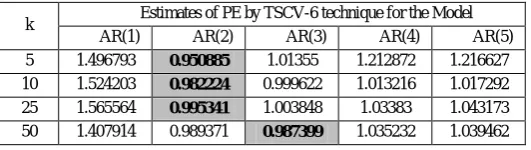
Table VI. Estimates of PE by TSCV-6 technique
k Estimates of PE by TSCV-6 technique for the Model
AR(1) AR(2) AR(3) AR(4) AR(5)
5 1.496793 0.950885 1.01355 1.212872 1.216627 10 1.524203 0.982224 0.999622 1.013216 1.017292 25 1.565564 0.995341 1.003848 1.03383 1.043173 50 1.407914 0.989371 0.987399 1.035232 1.039462
In the TSCV-6 technique, we chose the k value such that n 2 k
k −
is an integer and k≥5. The TSCV-6 technique
performs better for small values of k.
By the TSCV techniques, AR(2) model is the most appropriate model for the simulated data.
IV. CONCLUSIONS
In the present research work, we have investigated the use of time series cross-validation techniques for determining the order of autoregressive model. These time series cross-validation techniques are also useful for obtaining best model among the candidate models in time series forecasting. These time series cross-validation techniques are alternative to the model selection procedures such as Final Prediction Error (FPE) Criterion, Akaike Information Criterion (AIC), Bias-Corrected Akaike Information Criterion (AICc), Bayesian Information Criterion (BIC) and Minimum Description Length (MDL).
V. REFERENCES
[1] P. Burman, E. Chow, and D. Nolan, “A cross-validatory method for dependent data,” Biometrika, Vol. 84(2), pp. 351-358, June 1994.
[2] C.Bergmeir, R.J.Hyndman,andB.Koo,“Anoteon thevalidity of cross-validation for evaluating time series prediction,” Unpub lished.
[3] T. Hastie, R. Tibshirani, and J. Friedman, The Elements of Statis tical Learning: Data Mining, Inference, and Prediction, Springer-Verlag New York Publishing,
[4] S. Konishi and G. Kitagawa, Information Criteria and Statistical Modeling, Springer-Verlag New York Publishing, 2008, 1
2009, pp. 241-249.
st
[5] J. Racine, “Consistent cross-validatory model-selection for depe ndent data: hv-block cross-validation,” J. Econometrics, Vol. 99 (1), 2000, pp. 39-61.
ed., pp. 241.
[6]
[image:5.595.31.297.452.527.2]