Effective Use of Network Bandwidth Through the Implementation of the Forecaster Algorithm.

(1)

ABSTRACT

GILBERT, NICHOLAS DANIEL. Effective Use of Network Bandwidth Through the Implemen-tation of the Forecaster Algorithm. (Under the direction of Khaled Harfoush.)

(2)

c

(3)

Effective Use of Network Bandwidth Through the Implementation of the Forecaster Algorithm

by

Nicholas Daniel Gilbert

A thesis submitted to the Graduate Faculty of North Carolina State University

in partial fulfillment of the requirements for the Degree of

Master of Science

Computer Networking

Raleigh, North Carolina

2011

APPROVED BY:

Harry Perros Arne Nilsson

(4)

DEDICATION

(5)

ACKNOWLEDGEMENTS

(6)

TABLE OF CONTENTS

List of Tables . . . v

List of Figures . . . vi

Chapter 1 Introduction . . . 1

1.1 Problem Overview . . . 2

1.2 Contributions . . . 3

1.3 Organization of the Thesis . . . 4

Chapter 2 Previous Work and Current Theory . . . 6

2.1 One-Hop Path . . . 6

2.2 Multi-Hop Path . . . 7

2.3 Estimating Path Utilization . . . 7

Chapter 3 Forecaster Implementation . . . 9

3.1 Design . . . 9

3.2 Methods and Setup . . . 11

Chapter 4 Problems Encountered. . . 13

4.1 Timestamping . . . 13

4.2 Traffic Shaping . . . 15

4.3 New API . . . 16

4.4 Floating Point Calculations . . . 17

Chapter 5 Experimental Results . . . 19

5.1 Fixed Rate One-Hop No Cross Traffic . . . 19

5.2 Fixed Rate One-Hop Cross Traffic . . . 20

5.3 Poisson Rate One-Hop No Cross Traffic . . . 21

5.4 Poisson Rate One-Hop Cross Traffic . . . 22

Chapter 6 Conclusions and Future Work . . . 26

References. . . 27

Appendix . . . 29

Appendix A Code . . . 30

A.1 snet.c . . . 30

(7)

LIST OF TABLES

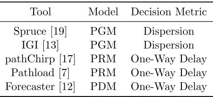
Table 1.1 Bandwidth Estimation Tools . . . 2

Table 5.1 Estimated Capacity . . . 25 Table 5.2 Estimated Capacity and Available Bandwidth with Cross Traffic of 500

(8)

LIST OF FIGURES

Figure 1.1 How inter-departure times relate to packet size and sending speed . . . . 4

Figure 3.1 Kernel Module Design . . . 10

Figure 3.2 Kernel Module Design . . . 11

Figure 4.1 Sending at a rate of 10 Mbps over 200 packets clock drift is visible . . . . 14

Figure 4.2 Sending at a rate of 10 Mbps over 1000 packets no clock drift is visible . 15 Figure 4.3 Sending at a rate of 10 Mbps low variation in spacing . . . 16

Figure 4.4 Sending at a rate of 100 Mbps low variation in spacing . . . 17

Figure 4.5 Sending at a rate of 500 Mbps high variation in spacing . . . 18

Figure 5.1 Time differences for 10 Mbps probe stream . . . 19

Figure 5.2 The average rate that the probe stream is being sent at for 10 Mbps stream 20 Figure 5.3 Time differences for 100 Mbps probe stream . . . 21

Figure 5.4 The average rate that the probe stream is being sent at for 100 Mbps stream . . . 22

Figure 5.5 Time differences for 10 Mbps probe stream . . . 23

Figure 5.6 The average rate that the probe stream is being sent at for 10 Mbps stream 23 Figure 5.7 Time differences for 10 Mbps probe stream . . . 24

Figure 5.8 The average rate that the probe stream is being sent at for 100 Mbps stream . . . 24

(9)

Chapter 1

Introduction

Bandwidth estimation of an Internet path is an important metric to measure for many different applications, and for evaluation of network performance. Because of the importance of this metric many tools have been created by the research community [23][1][21][9][6][20][11]. These tools can be split into three classes: congestion based, dispersion based, and delay based. Congestion based techniques are based on self-induced congestion, where the probe packets are sent at a rate that exceeds the available bandwidth. When sending at a rate larger than the available bandwidth there will be an increase in the One Way Delay (OWD) of the packets. By varying the rate of the probe stream and detecting when the OWD increases the tool will converge to the available bandwidth. This method is also known as iterative probing or the Probe Rate Model (PRM). The second technique, dispersion based, sends out packets with a specific gap and then measures the change in the dispersion of the packets on the receiving side. Assuming the capacity of the bottleneck link is known, the difference in the dispersion of the packets before and after the bottleneck link can be used to estimate the link load. Once we have the link load we can calculate the available bandwidth. The bottleneck neck link is both the narrow and tight link, and in order for this to method to work theses links must be the same. Where the narrow link is the link with the smallest capacity along the network path and the tight link is the link with the smallest available bandwidth. This method is also known as direct probing or the Probe Gap Model (PGM). The final technique is delay based and estimates the available bandwidth by looking at the delay experienced by each packet. If a packet experiences a higher delay when traversing the network then there is a high probability that the packet experienced queuing. By determine the number of packets that experience a larger delay the probability of a packet queuing can be calculated. We can then use the well-known formula for a one-hop path described in [1][2][12]

(10)

Table 1.1: Bandwidth Estimation Tools

Tool Model Decision Metric

Spruce [19] PGM Dispersion IGI [13] PGM Dispersion pathChirp [17] PRM One-Way Delay

Pathload [7] PRM One-Way Delay Forecaster [12] PDM One-Way Delay

Whereρi is the utilization of queue i andπ0i is the probability that there are no packets in the queue. Which allows us to estimate the utilization of the link, and once the utilization is the known the available bandwidth of the link can be calculated. This method is also known as isolated probing or the Probe Delay Model (PDM).

The PGM model is very sensitive to cross-traffic and has been proven inaccurate in [14]. PRM tools have the undesired effect of saturating the link that is being studied with a flood of probe packets. This means that a majority of the available bandwidth is used for probe packets and thus decrease the bandwidth available to other applications. Additional analysis of the PGM and PRM based tools is done in [14][19]. The PDM based model does not require any prior knowledge about the given path and does not make any simplifying assumptions about the current state of the network. All that is required in order to predict the available bandwidth is the ability to send out two probe streams. In [12] the PDM model Forecaster is proven to work in both theory and in simulation. The goal of this paper will be implementing the Forecaster Algorithm to run on hardware in order to test the accuracy of these claims.

1.1 Problem Overview

(11)

1.2 Contributions

We developed a tool that runs on physical hardware in order to validate the accuracy of the forecaster algorithm in a lab based environment. The algorithm was built into a Linux kernel module and tested in order to ensure that the algorithm works both in simulation as proven in [12] and on real physical hardware. In the process of building the tool we identified another state that had not been considered in the original paper. This state is when we have no cross traffic and are sending at a fixed rate; we should not see any packet queuing since there is no traffic in the network that would cause the packets to queue. By sending at a fixed rate you never cause any strain on the network, as long as you send at a rate that is lower than the capacity of the tight link. The other states that are described in [12] are:

1. Case 1: Base Case - No competing cross-traffic on any of the links

2. Case 2: The narrow link is the tight link

3. Case 3: The narrow link is not the tight link

4. Case 4: The high speed link in t he middle of the network path is the tight link

Our new state differs from all of these other states because there is no utilization of the link, and no queuing occurs for our case. When probes lead to queuing we know that we are either sending at a Poisson rate, or that there is enough cross traffic in the network in order to cause the fixed rate probes to queue. By testing this algorithm on an actual physical test bed we were able to identify some of the issues that can arise when using this algorithm. The first issue arises from the accuracy of the timestamps, and how inaccurate timestamps has a negative impact on the precision and variance of the predicted available bandwidth. The second issue has to deal with the accuracy of the algorithm on high speeds link. This issue arises from the level of precision needed in order to determine if a packet has queued on a high speed connection. For example when sending a 1500 byte packet probe stream out at 100 Mbps, on a 1000 Mbps link, we need to send out a packet every 120µs.

1500∗8bits

100M bps = 120µs (1.2)

(12)

on average one probe packet will be sent every 120 µs. This causes the accuracy of the traffic shaping function to come into play, and will be discussed further in the problems section. When sending packets out at higher rates the spacing in between the packets decreases at an exponential rate. This means that the function used for traffic shaping needs to be extremely

0 200 400 600 800 1000 1200 1400 1600

0 100 200 300 400 500

Inter-departure Time (microseconds)

Mbps

Inter-departure times vs Sending Speed

1500 Bytes 1200 Bytes 900 Bytes 600 Bytes 300 Bytes

Figure 1.1: How inter-departure times relate to packet size and sending speed

precise in order to accurately send packets out at the correct rate. The third problem has to deal with the packet size chosen for the probe packets. It can be seen in Figure 1.1 that by decreasing the packet size the number of packets sent in a given time interval must increase in order to achieve the same speeds. This once again means are traffic shaping function has to be extremely accurate in order to send out these smaller packets with smaller inter departure times.

1.3 Organization of the Thesis

(13)

(14)

Chapter 2

Previous Work and Current Theory

This research is based on the purposed Forecaster method [12] that uses a probe based approach in order to predict the end-to-end available bandwidth along a given network path, and the speed of the most congested link. This prediction method is unique in the fact that Forecaster does not require any prior knowledge about the given path and does not make any simplifying assumptions about the current state of the network. All that is required in order to predict the available bandwidth is the ability to send out two probe streams. Also in contrast to the Probe Rate Model [7][17], which sends probe streams at rates matching the available bandwidth, these probe streams are sent at rates much lower than the available bandwidth. Therefore Forecaster eliminates the problem of congesting the network path that you wish to study by sending out probe streams that will only take up a fraction of the available bandwidth. Each link along a given network path is modeled as a queue and using concepts from basic queuing theory the utilization along this path is estimated. The following sections give a quick summary of the work presented in [12] and the theory behind the forecaster algorithm.

2.1 One-Hop Path

With a one-hop path we know that we have a queuing system that only contains a single queue. According to [1][2][12] the utilization of this queue can be expressed as

ρi= 1−πi0 (2.1)

In addition we have to take in account for the probe packets that are being sent across the queue. The probe packets sent at rate r will utilize r/C of the links capacity where C is the capacity of the link. So now we know the effective utilization of the link to be

ρi(r) =min(1, ρi+

r Ci

(15)

2.2 Multi-Hop Path

In a multi-hop network we now must consider a sequence of links that are modeled as a number of successive queues. This adds another layer of complexity because in order to analysis this system we have to assume that the queues are uncorrelated, but this assumption will likely not hold true in all cases. Assuming that the queues are uncorrelated the utilization of the system can be expressed as

ρi(r) =min 

1,1− Y

1≤i≤H

1−

ρi+

r Ci



 (2.3)

There is correlation, but it has been shown that this correlation only delays convergence and that it does not lead to divergence [8]. As long as a large enough time slice is observed Equation 3 will hold true. Thus the end-to-end utilization of the network path can be expressed as

ρi(r) =min 1, H

X

i=1 ciri

!

(2.4)

It is also shown in [12] that the utilization of the network path can be further simplified to the following equation

ρi(r)≈min(1, c0+c1r) (2.5)

Where c0 and c1 are the coefficients of equation 4, and it is shown [12] that only the first two coefficients are significant.

2.3 Estimating Path Utilization

(16)

(17)

Chapter 3

Forecaster Implementation

In order to test the accuracy of Forecaster in non-simulated environment packets must be sent out while maintaining a high level of accuracy. In order to do this we will be operating inside the kernel space in order to avoid the overhead caused by running applications in the user space. The tool was built using a Linux Kernel Module, which will allow us to dynamically load are code into the Linux Kernel. By integrating our code into the Linux Kernel we will have access to many functions that are only available to kernel level applications. This includes functions that will allow us to pass packets directly to the Ethernet card (hard start xmit), thus bypassing the overhead of going through the Network Stack. Also included are very precise delay functions (udelay, mdelay). All of the testing and design was done for a link speed of 1 Gbps.

3.1 Design

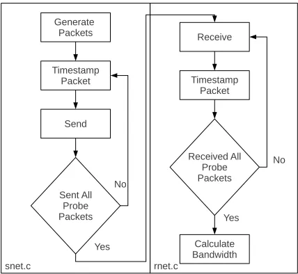
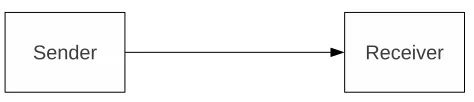
The tool consists of two Linux kernel modules, snet.c and rnet.c, one for the sender and one for the receiver. Each module needs to be loaded into the kernel using insmod and must have certain parameters specified when loaded. These parameters consist off

1. packetSize - the packet size (default: 1500 bytes)

2. numberOfPackets - number of packets to send/receive (default: 200)

3. numberOfRuns - number of times to send/receive the streams (default: 1)

4. rateOne - the rate of the first probe stream (default: 10 Mbps)

5. rateTwo - the rate of the second probe stream (default: 100 Mbps)

While the following three are specific to the sending computer (snet.c)

(18)

Figure 3.1: Kernel Module Design

2. mac address- the mac address of the destination computer

3. my eth - the Ethernet device on which to send the packet (default: eth0)

(19)

the packets in order to simulate a stream of packets at a given rate.

packetSize∗8

Rate =Delay (3.1)

This is then used as the rate for a Poisson process in order to generate the exponential inter-departure times; so that the probe stream we send out will take advantage of the PASTA property [22]. The problem with the traffic shaping function is that udelay [4] is a busy wait function, and this means that the CPU is unable to continue working on other tasks and instead must wait for udelay to finish. As soon as udelay finishes, the traffic shaping function might be interrupted by the CPU. This problem is something that will need to be addressed in the future through the use of the High Resolution Timers [3].

3.2 Methods and Setup

Figure 3.2: Kernel Module Design

(20)

(21)

Chapter 4

Problems Encountered

In order to test the effectiveness of the bandwidth signature algorithm [12] there are several key problems that need to be addressed.

4.1 Timestamping

(22)

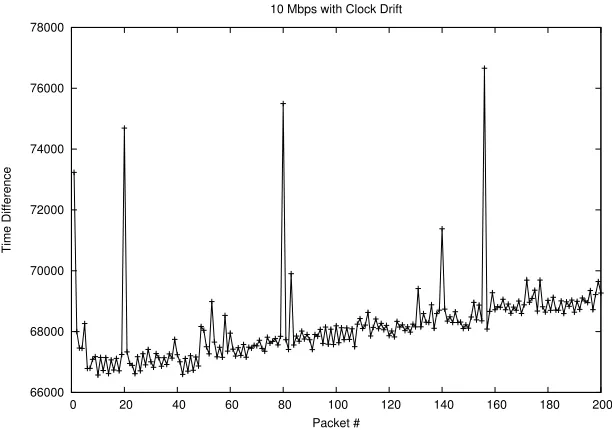
can be accounted for. Also the code has to be locked so that it only operates on a single CPU and out-of-order execution must be prevented by using a sterilizing instruction such as cupid. Calling the cpuid instruction forces every pending instruction to be executed before it is called, basically turning off out-of-order execution for this segment of code. These problems also affect the receiving computer and a new layer of complexity is added by clock drift. Even if both the sender and the receiver are operating at the same frequency there is still some clock drift that will occur. This clock drift means that over time the time stamp difference will change in value. In extreme cases you can actually see the clock drift occurring over a period of time.

66000 68000 70000 72000 74000 76000 78000

0 20 40 60 80 100 120 140 160 180 200

Time Difference

Packet # 10 Mbps with Clock Drift

Figure 4.1: Sending at a rate of 10 Mbps over 200 packets clock drift is visible

(23)

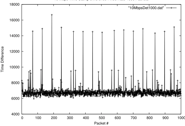
4000 6000 8000 10000 12000 14000 16000 18000

0 100 200 300 400 500 600 700 800 900 1000

Time Difference

Packet #

10 Mbps Time Stamp Difference Fixed Rate 1000 Packets

"10MbpsDet1000.dat"

Figure 4.2: Sending at a rate of 10 Mbps over 1000 packets no clock drift is visible

count into a time in seconds and nanoseconds. By converting to a unit of measurement that is not dependent on the current hardware this function will allow us to compare values without having to worry about clock drift.

4.2 Traffic Shaping

(24)

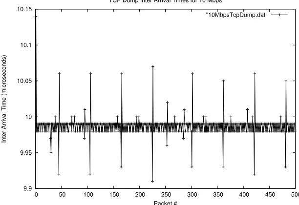
9.9 9.95 10 10.05 10.1 10.15

0 50 100 150 200 250 300 350 400 450 500

Inter Arrival Time (microseconds)

Packet #

TCP Dump Inter Arrival Times for 10 Mbps

"10MbpsTcpDump.dat"

Figure 4.3: Sending at a rate of 10 Mbps low variation in spacing

possible solution to this is to use the new High Resolution Timers that have been implemented in the new Linux Kernel. These timers allow for high precision and do not use a busy wait loop, and thus allow for other processes to utilize the CPU.

4.3 New API

(25)

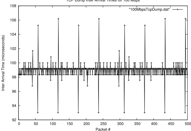
92 94 96 98 100 102 104 106 108

0 50 100 150 200 250 300 350 400 450 500

Packet #

"100MbpsTcpDump.dat"

Figure 4.4: Sending at a rate of 100 Mbps low variation in spacing

solution to this problem was to turn this feature off. The use of NAPI is completely optional and drivers will work perfectly fine without it. In order to disable this feature simply remove the current Ethernet driver from the kernel using modprobe r e1000 and then reinsert the driver using modprobe e1000 InterruptThrottleRate=0. The graph of the timestamp differences now conforms to a straight line when sending at a fixed rate. This is how the timestamp differences should look when sending slowly at a fixed rate because there should be no packet queuing.

4.4 Floating Point Calculations

(26)

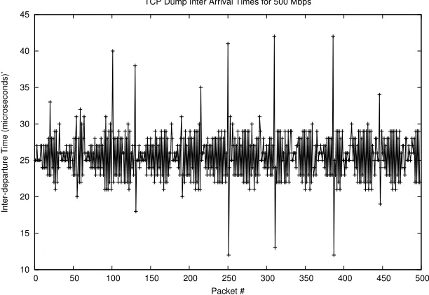
10 15 20 25 30 35 40 45

0 50 100 150 200 250 300 350 400 450 500

Inter-departure Time (microseconds)’

Packet #

Figure 4.5: Sending at a rate of 500 Mbps high variation in spacing

(27)

Chapter 5

Experimental Results

The following experiments were run with a packet size of 1500 bytes, probe rates of 10 Mbps and 100 Mbps, over a 1 Gbps link. We will look at the case where both of the probe streams are sent out at a fixed rate, and where both of the probe streams are sent out as a Poisson process.

5.1 Fixed Rate One-Hop No Cross Traffic

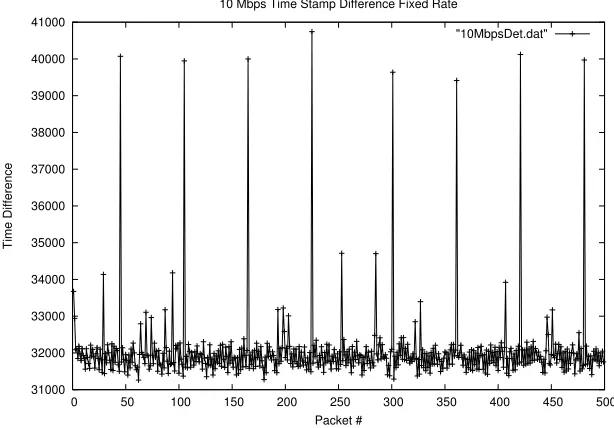
31000 32000 33000 34000 35000 36000 37000 38000 39000 40000 41000

0 50 100 150 200 250 300 350 400 450 500

Time Difference

Packet #

10 Mbps Time Stamp Difference Fixed Rate

"10MbpsDet.dat"

(28)

9.98 10 10.02 10.04 10.06 10.08 10.1 10.12 10.14 10.16

0 50 100 150 200 250 300 350 400 450 500

Inter Arrival Time (mircoseconds)

Time Totale Bytes / Total Time

"10MbpsRateCurve.dat"

Figure 5.2: The average rate that the probe stream is being sent at for 10 Mbps stream

In the 5.1 and 5.3 we can see how at a fixed rate the timestamp difference remains constant. While in 5.2 and 5.4 we can see that the tool is sending at the target rate. This is because with no cross traffic there is nothing on the network that would cause packets to queue. Because there is no packet queuing it will be impossible to measure the available bandwidth of the network path. When looking at the case where cross traffic exist on the network path this will no longer hold true, as long as the cross traffic simulates a Poisson process. If the cross traffic is sent at a fixed rate, then as long as the probe rate plus the cross traffic rate is less than the capacity of the link there should be no queuing. This is the new case where we are unable to predict that available bandwidth of the link, but it can be safely assumed the available bandwidth of the link is equal to the capacity of the link.

5.2 Fixed Rate One-Hop Cross Traffic

(29)

30000 31000 32000 33000 34000 35000 36000 37000 38000 39000 40000 41000

0 50 100 150 200 250 300 350 400 450 500

Time Difference

Packet #

100 Mbps Time Stamp Difference Fixed Rate - No Clock Drift

"100Mbps_Det.dat"

Figure 5.3: Time differences for 100 Mbps probe stream

can generate non uniform cross traffic.

5.3 Poisson Rate One-Hop No Cross Traffic

In the 5.5 and 5.7 we can see how when the probe packets are sent out as a Poisson process they experience queuing. This is caused by the fact that the Poisson process sends out the probe packets with only an average rate of 10 Mbps or 100 Mbps. The average rate we are sending out at can be seen in 5.6 and 5.8, and it can be seen that the Poisson process approximates 10 Mbps and 100 Mbps. So when packets are sent out in quick succession queuing occurs. When predicting how many packets queued out of a given probe stream a margin of error is needed. This is delta error is needed because of the variance in the traffic shaping function.

(30)

98.3 98.4 98.5 98.6 98.7 98.8 98.9 99 99.1

0 50 100 150 200 250 300 350 400 450 500

Packet # Total Bytes / Total Time

Average Rate

Figure 5.4: The average rate that the probe stream is being sent at for 100 Mbps stream

5.4 Poisson Rate One-Hop Cross Traffic

(31)

79000 80000 81000 82000 83000 84000 85000 86000 87000 88000 89000 90000

0 20 40 60 80 100 120 140 160 180 200

Time Difference

Packet #

10 Mbps Time Stamp Difference Poisson Rate

"10MbpsPos.dat"

5 6 7 8 9 10 11 12 13 14

0 20 40 60 80 100 120 140 160 180 200

Time Total Bytes / Total Time

(32)

375000 380000 385000 390000 395000 400000 405000 410000 415000

0 20 40 60 80 100 120 140 160 180 200

Time Difference

Packet #

100 Mbps Time Stamp Difference Poisson Rate

"100MbpsPos.dat"

90 100 110 120 130 140 150 160 170 180 190

0 20 40 60 80 100 120 140 160 180 200

Time Total Bytes / Total Time

(33)

Table 5.1: Estimated Capacity

Delta Error Estimated Capacity 95% CI

2 419.75 ±26.95

3 518.19 ±17.45

4 581.8 ±14.28

5 657.28 ±15.8

6 726.82 ±14.04

7 798.61 ±19.24

8 926.7 ±28.51

9 1068.17 ±33.69

10 1075.95 ±28.87

300 400 500 600 700 800 900 1000 1100 1200

2 4 6 8 10

Estimated Speed of Tight Link (C)

Delta Error (microseconds) Delta Error vs C

"C.dat"

Figure 5.9: Predicted Capacity of the link with different Delta Error

Table 5.2: Estimated Capacity and Available Bandwidth with Cross Traffic of 500 Mbps

Delta Error Estimated Capacity 95% CI Estimated Available Bandwidth 95% CI

8 1038 ±77.32 553.54 ± 43.86

(34)

Chapter 6

Conclusions and Future Work

(35)

REFERENCES

[1] A. Cabellos-Aparicio, F. Garcia, and J. Domingo-Pascual. A novel available bandwidth estimation and tracking algorithm. NOMS, 2008.

[2] Y. Cheng, V. Ravindran, A. Leon-Garcia, and H.-H. Chen. New exploration of packet-pair probing for available bandwidth estimation and traffic characterization. ICC, 2007.

[3] J. Corbet. The high-resolution timer api. 2006.

[4] J. Corbet, G. Kroah-Hartman, and A. Rubini. Linux Device Drivers. O’Reilly, third edition, 2005.

[5] Intel Corporation. Using the rdtsc instruction for performance monitoring. 1998.

[6] D. Croce, T. En Najjary, G. Urvoy Keller, and E. W. Biersack. Fast available bandwidth sampling for adsl links: rethinking the estimation for larger-scale measurements. PAM.

[7] C. Dovrolis and M. Jain. End-to-end available bandwidth: Measurement methodology, dynamics, and relation with tcp throughput. SIGCOMM.

[8] N. Duffield, J. Horowitz, D. Towsley, and F. Presti. Multicast-based inference of network-internal delay distribution. IEEE/ACM Transactions on Networking, 10:961–775, 2002.

[9] S. Ekelin, M. Nilsson, E. Hartikainen, A. Johnsson, J.-E. Mangs, B. Melander, and M. Bjorkman. Real-time measurement of end-to-end available bandwidth using kalman filtering. NOMS, 2006.

[10] Linux Foundation. Napi. 2009.

[11] E. Goldoni, G. Rossi, and A. Torelli. Assolo, a new method for available bandwidth estimation. ICIMP, 2009.

[12] K. Harfoush, M. Neginhal, and H. Perros. Measuring bandwidth signatures of network paths. Master’s thesis, North Carolina State University, 2007.

[13] N. Hu and P. Steenkiste. Evaluation and characterization of available bandwidth probing techniques. IEEE JSAC, 21(6):879–894, 2003.

[14] L. Lao, C. Dovrolis, and M. Y. Sanadidi. The probe gap model can underestimate the available bandwidth of multihop paths. Computer Communication Review, 36(5):29–34, 2006.

[15] S. B. Moon, P. Skelly, and D. Towsley. Estimation and removal of clock skew from network delay measurements. INFOCOM, 1999.

(36)

[17] V. Ribeiro, R. Riedi, R. Baraniuk, J. Navratil, and L. Cottrell. Pathchirp: Efficient available bandwidth estimation for network paths. PAM, 2003.

[18] A. Shipalov, C. D. Guerrero, M. A. Labrador, and M. Alzate. On the implementation of a capacity estimator for wireless ad hoc networks. SOUTHEASTCON, 2009.

[19] J. Strauss, D. Katabi, and F. Kaashoek. A measurement study of available bandwidth estimation tools. IMC, 2003.

[20] T. Tsugawa, C. L. T. Man, G. Hasegawa, and M. Murata. Inline network measurements: Implementation difficulties and their solutions. IEEE/IFIP E2EMON, 2007.

[21] Q. Wang and L. Cheng. Feat: Improving accuracy in end-to-end available bandwidth measurement. Globecom, 2006.

[22] R. Wolff. Poisson arrivals see time average. Operations Reasearch, 30:223–231, 1982.

(37)

(38)

Appendix A

Code

A.1 snet.c

#include <linux/module.h>

#include <linux/moduleparam.h>

#include <linux/kernel.h>

#include <linux/stat.h>

#include <linux/netdevice.h>

#include <linux/skbuff.h>

#include <linux/init.h>

#include <linux/in.h>

#include <linux/ip.h>

#include <linux/udp.h>

#include <linux/inetdevice.h>

#include <linux/inet.h>

#include <net/tcp.h>

#include <linux/proc_fs.h>

#include <linux/version.h>

#include <linux/jiffies.h>

#include <linux/sched.h>

#include <linux/delay.h>

#include <asm/delay.h>

#include <linux/time.h>

#include <linux/hrtimer.h>

#include <linux/ktime.h>

(39)

MODULE_LICENSE("GPL");

MODULE_AUTHOR("Nicholas Gilbert");

//this is the protocol that our packets will have

#define ETH_P_NET 0x1234

struct timeData{

//is it from rateOne or rateTwo

char type[2];

//structure to hold sender time information

struct timespec timeStampSender;

//structure to hold receiver time information

struct timespec timeStampReceiver;

};

//send a probe stream at rate

int sendProbeStream(int rate, int type);

int runNum=0;

//10 Mbps on a gig link 1500 byte packet

//big arrays

static int packetSize = 1500;

static int numberOfPackets = 100;

static int numberOfRuns = 1;

static int rateOne = 10;

static int rateTwo = 100;

static char *ip_address = "192.168.0.3";

static char *mac_address = "00:1B:21:2E:8F:F5";

//static char *mac_address = "00:1B:D4:94:B4:71";

static char *my_eth = "eth0";

(40)

static struct net_device *output;

static struct timespec tv;

static ktime_t delay;

/** Convert to micro-seconds */

static inline __u64 tv_to_us(const struct timeval *tv)

{

__u64 us = tv->tv_usec;

us += (__u64) tv->tv_sec * (__u64) 1000000;

return us;

}

module_param(packetSize, int, S_IRUSR | S_IWUSR | S_IRGRP | S_IWGRP);

module_param(numberOfPackets, int, S_IRUSR | S_IWUSR | S_IRGRP | S_IWGRP);

module_param(numberOfRuns, int, S_IRUSR | S_IWUSR | S_IRGRP | S_IWGRP);

module_param(rateOne, int, S_IRUSR | S_IWUSR | S_IRGRP | S_IWGRP);

module_param(rateTwo, int, S_IRUSR | S_IWUSR | S_IRGRP | S_IWGRP);

module_param(ip_address, charp, S_IRUSR | S_IWUSR | S_IRGRP | S_IWGRP);

module_param(mac_address, charp, S_IRUSR | S_IWUSR | S_IRGRP | S_IWGRP);

module_param(my_eth, charp, S_IRUSR | S_IWUSR | S_IRGRP | S_IWGRP);

int init_module(void) {

int retval=0;

printk(KERN_INFO "SENDER\n");

printk(KERN_INFO "Packet size: %dB\n", packetSize);

printk(KERN_INFO "Number of packets: %d\n", numberOfPackets);

printk(KERN_INFO "First Rate: %dMbs\n", rateOne);

printk(KERN_INFO "Second Rate: %dMbs\n", rateTwo);

//allocate memory for the list of Packets that we will be sending

packetList=(struct sk_buff_head *)

kmalloc(sizeof(struct sk_buff_head),GFP_KERNEL);

//loop to send the probe streams for the number of runs

//we are doing

while(runNum<numberOfRuns){

retval=sendProbeStream(rateOne,1);

if(retval==1)

(41)

else

printk(KERN_INFO "FALIURE_R1\n");

retval=sendProbeStream(rateTwo,2);

if(retval==1)

printk(KERN_INFO "SUCCESS_R2\n");

else

printk(KERN_INFO "FALIURE_R2\n");

runNum++;

set_current_state(TASK_INTERRUPTIBLE);

schedule_timeout(10 * HZ);

}

kfree(packetList);

return 0;

}

void cleanup_module(void) {

printk(KERN_INFO "END\n");

}

int sendProbeStream(int rate, int type) {

//skb buffer that holds the current packet we are creating

struct sk_buff *skb;

struct ethhdr *eth; //ethernet header

static struct iphdr *iph; //ip header

struct udphdr *udph; //udp header

u_char *payload; //the data section

//out data taht we want the packet to carry

static struct timeData *data;

//the device we are using to send these packets out on

struct in_device *in_dev;

int i; //count var

int paysize; //the size of the data segement of the packet

char * endptr; //used to change the mac format

(42)

skb_queue_head_init(packetList);

//calculate the reaminaing room for data in the packet

paysize=packetSize - (sizeof(struct ethhdr) + sizeof(struct iphdr)

+ sizeof(struct udphdr) + sizeof(struct timeData));

//loop to create packets

for (i=0; i < numberOfPackets; i++) {

//try to allocate memory for a new packet

skb=alloc_skb(packetSize, GFP_ATOMIC);

if (!skb) //if we do not succesfully alocate memory return 0

{

return 0;

}

//get our ouput device

output = dev_get_by_name(my_eth);

//check to make sure device is running

if(!netif_running(output))

return 0;

//need to add in the data before calculating the checksum

// setup pointers to where each header starts in the skb

skb_reserve(skb, sizeof(struct ethhdr));

eth=(struct ethhdr *) skb_push(skb, sizeof(struct ethhdr));

iph=(struct iphdr *) skb_put(skb, sizeof(struct iphdr));

udph=(struct udphdr *) skb_put(skb, sizeof(struct udphdr));

data=(struct timeData *) skb_put(skb, sizeof(struct timeData));

payload=(u_char *) skb_put(skb,paysize);

//fill ethernet header data

eth->h_proto = htons(ETH_P_NET);

//eth->h_proto=htons(ETH_P_IP);

//store the destination MAC address in the header

eth->h_dest[0]=simple_strtoul(mac_address ,&endptr, 16);

eth->h_dest[1]=simple_strtoul(mac_address+3 ,&endptr, 16);

(43)

//store the source MAC address in the header

eth->h_source[0]=output->dev_addr[0];

//fill ip header data

iph->tos=8; //type of service

//calc the total length of the packet

iph->tot_len=htons(sizeof(struct iphdr)

+ sizeof(struct udphdr) + paysize);

iph->frag_off=0; //turn fragmentation off

iph->ttl=32; //time to live

//mark this packet as using are custom protocol

iph->protocol=IPPROTO_UDP;

//set the checksum to 0 will recalculate after we have added

//the data

iph->check=0;

iph->ihl=5;

//Get the source address and store it in the ip header

if (output->ip_ptr) {

in_dev=output->ip_ptr;

if (in_dev->ifa_list) {

iph->saddr=in_dev->ifa_list->ifa_address;

}

iph->daddr=in_aton(ip_address); //Destination address is stored

iph->version=4; //version

//fill udp header data

udph->source=htons(1101);

udph->dest=htons(1101);

udph->len=htons(paysize + sizeof(struct udphdr));

(44)

//fill sock buff header data

skb->protocol=__constant_htons(ETH_P_NET);

skb->mac.raw=((u8 *)eth);

//set the skb device to the output

skb->dev=output;

skb->pkt_type=PACKET_OUTGOING; //mark this as an outgoing packet

//Depending on which probe stream this is add in a flag

if(rate==rateOne && type==1)

{

data->type[0]=’T’;

data->type[1]=’S’;

data->type[2]=’1’;

}

else if(rate==rateTwo && type==2)

{

data->type[0]=’T’;

data->type[1]=’S’;

data->type[2]=’2’;

}

//go ahead and calculate the checksum

iph->check=ip_fast_csum((void *)iph,iph->ihl);

//add skb to the packet list

skb_queue_head(packetList,skb);

}

printk(KERN_INFO "\n");

//loop to send packets and put timestamps into there data section

skb=skb_dequeue(packetList);

//use ktime_get_ts for traffic shaping

i=0;

//do_gettimeofday(&ctv);

(45)

while (skb != NULL) {

//do_gettimeofday(&tv);

//getnstimeofday(&tv);

ktime_get_ts(&tv);

((struct timeData *)((skb->data)+42))->timeStampSender=tv;

//LOCK

netif_tx_lock_bh(output);

if(output->hard_start_xmit(skb, output)){

printk(KERN_INFO "PACKET FAIL #%d, ",i);

//we need to requeue the packet

skb_queue_head(packetList,skb);

i--;

}

//UNLOCK

netif_tx_unlock_bh(output);

skb=skb_dequeue(packetList);

//delay before we send out the next packet

if(type==1){

//udelay(iTime1[i]);

//udelay(iTime11[i+(runNum*200)]);

udelay((int)packetSize*8/rateOne);

}

else

//udelay(iTime6[i]);

//udelay(iTime12[i+(runNum*200)]);

udelay((int)packetSize*8/rateTwo);

i++;

}

printk(KERN_INFO "\n");

return 1;

}

A.2 rnet.c

#include <linux/module.h>

(46)

#include <linux/kernel.h>

#include <linux/stat.h>

#include <linux/netdevice.h>

#include <linux/skbuff.h>

#include <linux/init.h>

#include <linux/in.h>

#include <linux/ip.h>

#include <linux/udp.h>

#include <linux/inetdevice.h>

#include <linux/inet.h>

#include <net/tcp.h>

#include <linux/proc_fs.h>

#include <linux/version.h>

#include <linux/jiffies.h>

MODULE_LICENSE("GPL");

MODULE_AUTHOR("Nicholas Gilbert");

//this is the protocol that our packets will have

#define ETH_P_NET 0x1234

#ifndef htonll

#ifdef _BIG_ENDIAN

#define htonll(x) (x)

#define ntohll(x) (x)

#else

#define htonll(x) ((((uint64_t)htonl(x)) << 32) + htonl(x >> 32))

#define ntohll(x) ((((uint64_t)ntohl(x)) << 32) + ntohl(x >> 32))

#endif

struct timeData{

char type[2]; //is it from rateOne or rateTwo

//long int timeStampSender;

//long int timeStampReceiver;

(47)

struct timespec timeStampReceiver;

};

typedef struct {

signed int whole;

signed int denominator;

signed int remainder;

}fpNumber;

struct bandData{

fpNumber A; //avaliable bandwidth

fpNumber C; //capacity

fpNumber c1;

fpNumber c0;

};

//funcitons for floating point calculations

fpNumber fpDivide(int n1, int n2);

fpNumber fpDiv(fpNumber n1, int n2);

fpNumber fpD(fpNumber n1, fpNumber n2);

fpNumber fpMultiply(fpNumber n1, fpNumber n2);

fpNumber fpMulti(int n1, fpNumber n2);

fpNumber fpSubtraction(fpNumber n1, fpNumber n2);

fpNumber fpSub(int n1, fpNumber n2);

fpNumber fpAdd(fpNumber n1, fpNumber n2);

fpNumber fpSimplfy(fpNumber n);

int gcd(int n1, int n2);

void printFp(fpNumber n);

void calcBand(void); //calculate the avaliable bandwidth

int test_pack_rcv(struct sk_buff *skb, struct net_device *dev,

struct packet_type *pt, struct net_device *dev1);

void subtract_timespec(struct timespec *a,

struct timespec *b, struct timespec *diff);

struct timespec minTimespec(struct timespec *a);

(48)

static int packetSize = 1500;

static int numberOfPackets = 100;

static int numberOfRuns = 1;

static int rateOne = 10;

static int rateTwo = 100;

static struct sk_buff_head *packetList;

static struct sk_buff_head *packetList2;

static struct timespec tv;

//the difference in the timestamps

struct timespec *timeDiff, *timeDiff2, *timeDiff3;

static struct packet_type new_protocol = { htons(ETH_P_NET), NULL,

&test_pack_rcv, NULL, NULL, NULL };

module_param(packetSize, int, S_IRUSR | S_IWUSR | S_IRGRP | S_IWGRP);

module_param(numberOfPackets, int, S_IRUSR | S_IWUSR | S_IRGRP | S_IWGRP);

module_param(numberOfRuns, int, S_IRUSR | S_IWUSR | S_IRGRP | S_IWGRP);

module_param(rateOne, int, S_IRUSR | S_IWUSR | S_IRGRP | S_IWGRP);

module_param(rateTwo, int, S_IRUSR | S_IWUSR | S_IRGRP | S_IWGRP);

int init_module(void) {

//allocate first probe stream list

packetList = (struct sk_buff_head *)

//allocate second probe stream list

packetList2 = (struct sk_buff_head *)

skb_queue_head_init(packetList2);

//allocate mem for time Difference for algotrithm calculations

timeDiff = kmalloc(numberOfPackets*sizeof(struct timespec),GFP_KERNEL);

timeDiff2 = kmalloc(numberOfPackets*sizeof(struct timespec),GFP_KERNEL);

//add our protocol

(49)

return 0;

}

void cleanup_module(void) {

//we need to cal avaliable bandwidth and then print out the result

//test to make sure that we have received all of the packets

//that we were suppose to recieve

if(!skb_queue_empty(packetList) && !skb_queue_empty(packetList2))

{

if(skb_queue_len(packetList)==

numberOfPackets && skb_queue_len(packetList2)==numberOfPackets){

//calcBand();

//printk(KERN_INFO "calcBand()\n");

}

else{

printk(KERN_INFO "PACKET LIST NOT FULL\n");

printk(KERN_INFO "R1:%u R2:%u\n",skb_queue_len(packetList),

skb_queue_len(packetList2));

}

dev_remove_pack(&new_protocol);

kfree(packetList);

kfree(packetList2);

}

else if(skb_queue_empty(packetList) && skb_queue_empty(packetList2))

{

//printk(KERN_INFO "PROBE STREAM EMPTY\n");

kfree(packetList);

kfree(packetList2);

}

else

{

printk(KERN_INFO "R1:%u R2:%u\n",skb_queue_len(packetList),

skb_queue_len(packetList2));

kfree(packetList);

(50)

}

kfree(timeDiff);

kfree(timeDiff2);

printk(KERN_INFO "END\n");

}

int test_pack_rcv(struct sk_buff *skb, struct net_device *dev,

struct packet_type *pt, struct net_device *dev1) {

if(skb->protocol == __constant_htons(ETH_P_NET))

{

//do_gettimeofday(&tv);

//getnstimeofday(&tv);

ktime_get_ts(&tv);

((struct timeData *)(skb->data+28))->timeStampReceiver = tv;

if(((struct timeData *)(skb->data+28))->type[2]==’1’){

//printk(KERN_INFO "TS1/n");

//add the packet to the current packetList

skb_queue_tail(packetList, skb);

}

else if(((struct timeData *)(skb->data+28))->type[2]==’2’){

//printk(KERN_INFO "TS2/n");

//add the packet to the current packetList

skb_queue_tail(packetList2, skb);

}

else

printk(KERN_INFO "PACKET HEADER CORRUPT\n");

if(skb_queue_len(packetList)==

numberOfPackets && skb_queue_len(packetList2)==numberOfPackets){

//printk(KERN_INFO "Run#%u:\n",runNum);

calcBand();

skb_queue_head_init(packetList2);

if(runNum>(numberOfRuns-1))

cleanup_module();

(51)

}

return skb->len;

}

return 0;

}

void calcBand(void)

{

struct sk_buff *skb; //holds the current packet we are looking at

struct bandData results;

int numQueue = 0;

int i=0,j=0; //counting var

fpNumber pr1={0,0,0},pr2={0,0,0};

struct timespec minTD;

//first need to cal p(r1) & p(r2)

//calc p(r1)

//make sure to init timeDiff arrays to 0

for(i=0;i<numberOfPackets;i++){

timeDiff[i].tv_sec=0;

timeDiff2[i].tv_sec=0;

timeDiff[i].tv_nsec=0;

timeDiff2[i].tv_nsec=0;

}

i=0;

skb = skb_dequeue(packetList);

if(skb==NULL)

return;

//loop to calculate the min time diff

for(i=0;i<(numberOfPackets);i++)

{

subtract_timespec(&((struct timeData *)(skb->data+28))->timeStampSender,

&((struct timeData *)(skb->data+28))->timeStampReceiver, &tv);

timeDiff[i]=tv;

(52)

}

minTD = minTimespec(timeDiff);

//printk(KERN_INFO "MIN#1:%ld",minTD.tv_nsec);

/* for(i=0;i<(numberOfPackets);i++)

{

//if timeDiff is greater then the min then packet queue

//need to determine margin of error so that timeDiff does not have

//to be exact, start with error of 0

//printk(KERN_INFO "TIMEDIFF#%u: %ld %ld\n",i,timeDiff[i].tv_sec,

timeDiff[i].tv_nsec);

if((timeDiff[i].tv_nsec>(minTD.tv_nsec+9000)))

numQueue++;

}

pr1.remainder = numQueue;

pr1.denominator = numberOfPackets;*/

//printk(KERN_INFO "PR1 ");

//printFp(pr1);

//printk(KERN_INFO "R1 Queue: %u ,",numQueue);

//calc p(r2)

numQueue=0; //reset queue number

i=0;

skb = skb_dequeue(packetList2);

if(skb==NULL)

return;

//loop to calculate the min time diff

{

subtract_timespec(&((struct timeData *)(skb->data+28))->timeStampSender,

&((struct timeData *)(skb->data+28))->timeStampReceiver, &tv);

timeDiff2[i]=tv;

skb = skb_dequeue(packetList2);

}

minTD = minTimespec(timeDiff2);

(53)

/* for(i=0;i<(numberOfPackets);i++)

{

//need to determine margin of error so that timeDiff does not have

//to be exact, start with error of 0

//printk(KERN_INFO "TIMEDIFF2#%u: %ld %ld\n",i,timeDiff2[i].tv_sec,

timeDiff2[i].tv_nsec);

if((timeDiff2[i].tv_nsec>(minTD.tv_nsec+9000)))

numQueue++;

}

pr2.denominator = numberOfPackets;*/

//printk(KERN_INFO "PR2 ");

//printFp(pr2);

//printk(KERN_INFO "R2 Queue: %u ,",numQueue);

//now that we have p(r1) & p(r2) we can calculate info we need

/*c1 = (pr2-pr1)/(rateTwo-rateOne);

data->C = 1/c1;

c0 = pr1-(rateOne*c1);

data->A = (1-c0)/c1;*/

/* if(((rateTwo-rateOne)>0) && pr1.remainder!=pr2.remainder){

results.c1 = fpDiv(fpSubtraction(pr2,pr1),(rateTwo-rateOne));

results.C.whole = 0;

results.C.remainder = results.c1.denominator;

results.C.denominator = results.c1.remainder;

results.C = fpSimplfy(results.C);

results.c0 = fpSubtraction(pr1,fpMulti(rateOne,results.c1));

//printFp(fpSub(1,results.c0));

results.A = fpD(fpSub(1,results.c0),results.c1);

//printFp(results.c1);

printk(KERN_INFO "C: ");

printFp(results.C);

printk(KERN_INFO "A: ");

printFp(results.A);

(54)

//calculate the other

for(j=1;j<11;j++){

numQueue=0;

{

//need to determine margin of error so that

//timeDiff does not have to be exact, start with error of 0

//printk(KERN_INFO "TIMEDIFF#%u: %ld %ld\n",i,timeDiff[i].tv_sec,

timeDiff[i].tv_nsec);

if((timeDiff[i].tv_nsec>(minTD.tv_nsec+(j*1000))))

numQueue++;

}

pr1.denominator = numberOfPackets;

numQueue=0;

{

//need to determine margin of error so that

//timeDiff does not have to be exact, start with error of 0

//printk(KERN_INFO "TIMEDIFF2#%u: %ld %ld\n",i,timeDiff2[i].tv_sec,

timeDiff2[i].tv_nsec);

if((timeDiff2[i].tv_nsec>(minTD.tv_nsec+(j*1000))))

numQueue++;

}

pr2.denominator = numberOfPackets;

if(((rateTwo-rateOne)>0) && pr1.remainder!=pr2.remainder){

results.c1 = fpDiv(fpSubtraction(pr2,pr1),(rateTwo-rateOne));

results.C.whole = 0;

results.C.remainder = results.c1.denominator;

results.C.denominator = results.c1.remainder;

results.C = fpSimplfy(results.C);

results.c0 = fpSubtraction(pr1,fpMulti(rateOne,results.c1));

//printFp(fpSub(1,results.c0));

(55)

printk(KERN_INFO "C%d: ",j);

printFp(results.C);

printk(KERN_INFO "A%d: ",j);

printFp(results.A);

printk(KERN_INFO "\n");}

}

fpNumber fpDivide(int n1, int n2){

fpNumber result;

result.denominator = n2;

result.whole = n1/n2;

result.remainder = n1%n2;

return fpSimplfy(result);

}

fpNumber fpDiv(fpNumber n1, int n2){

fpNumber result;

result.whole = 0;

result.denominator = n1.denominator * n2;

result.remainder = n1.remainder;

return fpAdd(fpDivide(n1.whole,n2),result);

}

fpNumber fpD(fpNumber n1, fpNumber n2){

n1.remainder += n1.whole*n1.denominator;

n1.whole=0;

n2.whole = n2.denominator;

n2.denominator=n2.remainder;

n2.remainder=n2.whole;

n2.whole=0;

return fpMultiply(n1,n2);

(56)

fpNumber fpMultiply(fpNumber n1, fpNumber n2){

n1.whole = 0;

n2.whole = 0;

n1.remainder *= n2.remainder;

n1.denominator *= n2.denominator;

return fpSimplfy(n1);

}

fpNumber fpMulti(int n1, fpNumber n2){

fpNumber result={n1,1,0};

if(n1==1)

return n2;

return fpMultiply(result,n2);

}

fpNumber fpSubtraction(fpNumber n1, fpNumber n2){

n1.whole = 0;

n2.whole = 0;

if(n1.denominator==n2.denominator){

n1.remainder -= n2.remainder;}

else{

n1.remainder *= n2.denominator;

n1.remainder -= n2.remainder;}

}

fpNumber fpSub(int n1, fpNumber n2){

fpNumber temp = {n1,1,0};

return fpSubtraction(temp, n2);

(57)

fpNumber fpAdd(fpNumber n1, fpNumber n2){

n1.whole = 0;

n2.whole = 0;

if(n1.denominator==n2.denominator){

n1.remainder += n2.remainder;}

else{

n1.remainder += n2.remainder;}

}

fpNumber fpSimplfy(fpNumber n){

fpNumber result=n;

int g;

while(result.remainder<0&&((result.remainder*-1)>

result.denominator)){

result.whole--;

result.remainder += result.denominator;}

while(result.remainder>=result.denominator){

result.whole++;

result.remainder -= result.denominator;}

g = gcd(result.denominator,result.remainder);

//printk(KERN_INFO "GCD:%u\n",g);

result.remainder /= g;

result.denominator /= g;

return result;

}

int gcd(int n1, int n2){

int t;

if(n1<n2){

t=n1;

(58)

n2=t;}

while(n2 != 0){

t = n2;

n2 = n1%n2;

n1 = t;}

return n1;

}

void printFp(fpNumber n){

printk(KERN_INFO "%i %i/%i ",n.whole,n.remainder,n.denominator);

}

void subtract_timespec(struct timespec *a, struct timespec *b,

struct timespec *diff)

{

//printk(KERN_INFO "Sender:%ld Recevier:%ld",a->tv_sec,b->tv_sec);

if(a->tv_sec>b->tv_sec){

//printk(KERN_INFO "Sender > Reciever");

diff->tv_nsec = a->tv_nsec-b->tv_nsec;

if(diff->tv_nsec<0){

diff->tv_nsec += 1000000000;

diff->tv_sec = a->tv_sec-b->tv_sec-1;}

else

diff->tv_sec = a->tv_sec-b->tv_sec;}

else if(a->tv_sec<b->tv_sec){

//printk(KERN_INFO "Sender < Reciever");

diff->tv_nsec = b->tv_nsec-a->tv_nsec;

if(diff->tv_nsec<0){

diff->tv_nsec += 1000000000;

diff->tv_sec = b->tv_sec-a->tv_sec-1;}

else

diff->tv_sec = b->tv_sec-a->tv_sec;}

else{

diff->tv_sec=0;

if(a->tv_nsec<b->tv_nsec){

(59)

diff->tv_nsec = b->tv_nsec-a->tv_nsec;}

else{

//printk(KERN_INFO "Reciever < Sender");

diff->tv_nsec = a->tv_nsec-b->tv_nsec;}}

}

struct timespec minTimespec(struct timespec *a)

{

int i;

struct timespec min=a[0];

for(i=0;i<numberOfPackets;i++)

if(min.tv_nsec>a[i].tv_nsec)

min=a[i];

return min;