ABSTRACT
BENNER, STEVEN. Development of a Coarse-Grained Model of Chitosan for Predicting Solution Behavior. (Under the direction of Dr. Carol K. Hall).
We have developed a new, implicit-solvent, coarse-grained model of chitosan designed for use in discontinuous molecular dynamics (DMD) simulations. The parameters for this model were developed using a multi-scale modeling approach based on explicit-solvent, atomistic simulations. We used our coarse-grained model of chitosan to predict self-assembly behavior as a function of the degree of acetylation (DA) and amount of hydrophobic modification (based on alkanes). The self-assembly of chitosan was studied to determine its potential as a biocompatible material for targeted drug delivery and oil spill remediation.
is a saturation density of longer modification chains, above which there is no improvement in performance as an oil dispersant additive. We also determined that longer modification chains more effectively penetrate into oil droplets, resulting in a deformation of their shape which was quantified by measuring the asphericity of the oil droplets.
Next we performed a multi-scale modeling procedure to develop a more detailed coarse-grained model of chitosan. The model contains two different monomer types which allow the investigation of systems with varying DA: protonated glucosamine (GlcN+
) and N-acetylglucosamine (GlcNAc). Each monomer is modeled with three coarse-grained sites; the chitosan chain length was set to 100 monomers. The results showed increased association between chitosan chains with increasing DA. Increasing the DA from 10% to 50% resulted in the formation of percolated chitosan networks earlier in time for each increase in DA. Furthermore, the networks formed at DA’s of 20% and higher contained all of the chains in the system. The number of monomer-monomer interactions also increased with increasing DA, indicating a stronger network with more structural integrity. Under dilute solution conditions, our model closely matches the radius of gyration and persistence lengths of chitosan reported in experiments as a function of DA. Overall, we have shown that the behavior of our coarse-grained model conceptually matches several behaviors observed experimentally.
show that the sequence of acetylated monomers can have a significant impact on the rate of network formation, particularly at low DA. At 10% DA, we showed that only a blocky sequence of acetylated monomers leads to a stable percolated structure while random and evenly spaced sequences do not. For DA’s of 20% and higher, the blocky sequences form a percolated network the fastest, followed by random, and then evenly spaced sequences. We also showed that the pore size distribution of the chitosan networks can be adjusted based on both the DA and the monomer sequence. Increasing DA leads to networks with larger pores due to the increased hydrophobic association between chains. Blocky sequences of acetylated monomers lead to networks with larger pores than random and evenly spaced sequences at a set DA. These different pore size distributions lead to changes in the diffusion of molecules inside the network. We show that networks of chitosan at high DA allow diffusion of larger molecules than networks at low DA due to the increase in pore size.
Development of a Coarse-Grained Model of Chitosan for Predicting Solution Behavior
by
Steven William Benner
A dissertation submitted to the Graduate Faculty of North Carolina State University
in partial fulfillment of the requirements for the degree of
Doctor of Philosophy
Chemical Engineering
Raleigh, North Carolina 2016
APPROVED BY:
_______________________________ ______________________________
Dr. Carol K Hall Dr. Jan Genzer
Committee Chair
________________________________ ________________________________ Dr. Erik Santiso Dr. Saad Khan
ii DEDICATION
This dissertation is dedicated to my parents, Bill and Susan Benner, my brother, Glenn
Benner, and my fiancé, Maggie Fuentes. Thank you for keeping me motivated throughout
this process and keeping things in perspective for me when I needed it. Your support has
helped me more than I can explain, and I could not imagine going through this process
iii BIOGRAPHY
iv ACKNOWLEDGMENTS
I would like to express my gratitude towards my Ph.D. committee who has had a tremendous impact on my time at NC State. First I would like to thank my advisor Dr. Carol Hall for overseeing my graduate career and providing many insightful discussions about my research projects and development as a scientist. Our interaction over the past five years has helped shape my professional career and given me perspective on future goals to pursue. She always provided the guidance to keep me motivated while giving me the freedom to pursue directions that I found stimulating. I look forward to the many discussions we will continue to have in the future. I would also like to thank Dr. Jan Genzer for always taking the time to meet with me to discuss ideas and help give me direction. I am also grateful for the help of Dr. Erik Santiso for discussion of modeling and simulation strategies throughout my Ph.D. work. I would also like to thank Dr. Saad Khan and Dr. Maurice Balik for agreeing to join my committee and offering their input to my work. Finally, I would like to thank Dr. Vijay John and Dr. Pradeep Venkataraman for many insightful discussions throughout our collaboration.
v I would like to thank all of the past and present Hall group members that I have had the pleasure of working with over the years. A special thanks to past group members Emily Curtis for helping me get started with research and finding my bugs early on, and Dave Latshaw for welcoming me into the group and for a number of entertaining workout discussions and training sessions. I would like to thank senior group members David Rutkowski and Binwu Zhao for plenty of laughter and conversation throughout our years here. I would also like thank the post docs Xingqing Xiao and Qing Shao for their expertise and guidance. A final thanks to the younger group members: Kye Won Wang, Yiming Wang, Ryan Maloney, and Amelia Chen. Keep up the good work.
vi TABLE OF CONTENTS
LIST OF TABLES ... ix
LIST OF FIGURES ... xi
CHAPTER 1 ... 1
Motivation and Overview ... 1
1.1 Motivation ... 2
1.2 Overview ... 5
1.2.1 Simulation Study of Hydrophobically-modified Chitosan as an Oil Dispersant Additive ... 5
1.2.2 Development of a Coarse-Grained Model of Chitosan for Predicting Solution Behavior .... 6
1.2.3 Effect of Monomer Sequence and Degree of Acetylation on the Self-assembly and Porosity of Chitosan Networks in Solution ... 7
1.2.4 Nanoparticle Induced Assembly of Hydrophobically-Modified Chitosan ... 8
1.2.5 Future Work ... 9
1.3 Publications ... 10
1.4 References ... 11
CHAPTER 2 ... 19
Simulation Study of Hydrophobically-modified Chitosan as an Oil Dispersant Additive ... 19
2.1 Introduction ... 21
2.2 Methods ... 26
2.3 Results ... 33
vii
2.5 Acknowledgements ... 48
2.6 References ... 49
CHAPTER 3 ... 67
Development of a Coarse-Grained Model of Chitosan for Predicting Solution Behavior ... 67
3.1 Introduction ... 69
3.2 Methods ... 75
3.3 Results ... 80
3.4 Discussion and Conclusions ... 90
3.5 Acknowledgements ... 94
3.6 References ... 95
CHAPTER 4 ... 116
Effect of Monomer Sequence and Degree of Acetylation on Self-Assembly and Porosity of Chitosan Networks in Solution ... 116
4.1 Introduction ... 118
4.2 Methods ... 124
4.3 Results ... 127
4.4 Discussion and Conclusions ... 133
4.5 Acknowledgements ... 137
4.6 References ... 138
CHAPTER 5 ... 157
viii
5.1 Introduction ... 159
5.2 Methods ... 163
5.3 Results ... 167
5.4 Discussion and Conclusions ... 176
5.5 Acknowledgements ... 180
5.6 References ... 181
CHAPTER 6 ... 196
Conclusions and Future Work ... 196
6.1 Conclusions ... 197
6.2 Future Recommendations ... 201
6.2.1 Ionic Cross-Linking of Chitosan Hydrogels ... 201
6.2.2 pH Induced Swelling of Chitosan Hydrogels ... 202
6.2.3 Drug Delivery of Doxorubicin and Gemcitabine Using Chitosan Hydrogels ... 203
6.3 References ... 207
ix LIST OF TABLES
Table 2.1. Interaction energies between each type of sphere ... 64
Table 2.2. Average asphericity of oil aggregates for systems of HMCs with various modification densities and modification chain lengths for ϕhmc = 0.5 ... 65
Table 2.3. Percent increase in oil SASA in systems of 4% modified HMCs with 5 and 15-sphere modification chains at ϕhmc = 0.5 over systems of oil only ... 66
Table 3.1. Hard-sphere diameter, well/shoulder boundaries, and well/shoulder depths between each coarse-grained type ... 113
Table 3.2. Average distance between monomers along the chain in all-atom (AA) and coarse-grained (CG) simulations. Distances reported for chitosan are between two type 1 sites, and distances reported for chitin are between two type 4 sites. Nearest neighbors refer to monomers that are next to each other, next-nearest neighbors refer to monomers separated by one monomer, and next-next-nearest neighbors refer to monomers separated by two
monomers, along the chain. ... 114
Table 3.3. Radius of gyration (Rg) and persistence length (Lp) of 800-mer chitosan chains with different DA ... 115
x interaction potential, and σx refers to the separation distance corresponding
to each discontinuity. ... 210
Table A2. Interaction energies between each coarse-grained site. Type i and Type i refer to the coarse-grained type, εtotal refers to the total number of
square-wells/square-shoulders in the interaction potential, and εx refers to the depth
of each well. ... 213
Table A3. Bond and pseudobond distances between backbone sites on chitosan
(between two type 1 spheres) and chitin chains (between two type 4 spheres). Type i and Type j refer to the coarse-grained type. A bond type of “a” indicates a nearest-neighbor bond, a bond type of “b” indicates a next-nearest-neighbor pseudobond, and a bond type of “c” indicates a next-next-nearest neighbor pseudobond. The min distance is the minimum bond
distance and the max distance is the maximum bond distance. ... 216
Table A4. Bond and pseudobond distances between coarse grained sites. Type i and Type j refer to the coarse-grained type. A bond type of “a” indicates a bond, a bond type of “b” indicates a pseudobond. The min distance is the
minimum bond distance and the max distance is the maximum bond
xi LIST OF FIGURES
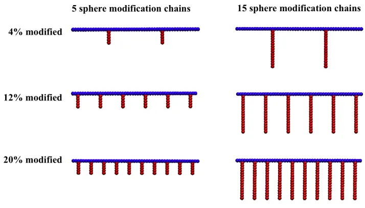
Figure 2.1. Schematic diagram showing the different architecture HMCs used in
simulations of systems containing HMCs and oil ... 54
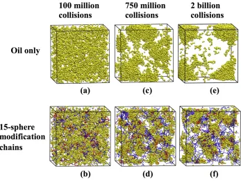
Figure 2.2. Snapshots of oil aggregation during simulations of systems containing oil only and oil + 4% modified HMCs with 15-sphere modification chains where ϕhmc = 0.5. Chitosan spheres are blue, modification spheres are red, and oil
spheres are yellow. ... 55
Figure 2.3. Effect of HMC modification density on ability of HMCs with (a) 5 and (b) 15-sphere modification chains to prevent oil aggregation for ϕhmc = 0.5 ... 56
Figure 2.4. Percent increase in oil SASA for HMCs with (a) 5 or (b) 15-sphere
modification chains and varying modification density ... 57
Figure 2.5. Oil aggregate size distributions over time using 20% modified HMCs with (a) 5 or (b) 15-sphere modification chains at ϕhmc = 0.5 ... 58
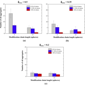
Figure 2.6. Oil aggregate size distributions at the end of simulations using 20%
modified HMCs with 5 or 15-sphere modification chains with ϕhmc = (a) 0.5,
(b) 0.35, and (c) 0.2 ... 59
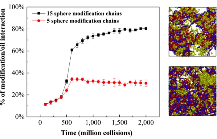
xii Figure 2.8. Percentage of modification spheres interacting with oil spheres during
simulations with 20% modified HMCs with 5 and 15-sphere modification chains ... 61
Figure 2.9. Snapshots of networks formed by (a) unmodified chitosan, (b) 20% modified HMCs with 5-sphere modification chains, and (c) 20% modified HMCs with 15-sphere modification chains. Chitosan spheres are in blue and
modification spheres are in red. ... 62
Figure 2.10. Oil aggregate size distributions comparing systems of HMCs with (a) few long modification chains and (b) many short modification chains at ϕhmc = 0.5
... 63
Figure 3.1. Coarse-graining scheme for different monomer types. Numbers refer to the coarse-grained site type. ... 102
Figure 3.2. Atomistic and coarse-grained representations of a chitosan chain consisting of 6 GlcN+ monomers ... 103
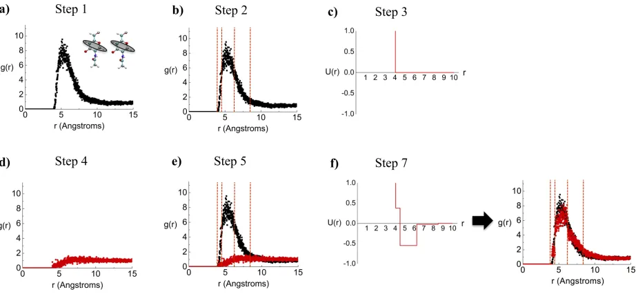
xiii after the first iteration, f) final discontinuous potential (left) and overlay of the final coarse-grained RDF (red) and atomistic RDF (black) (right). ... 104
Figure 3.4. Comparison of atomistic (black) and coarse-grained (red) radial distribution functions between coarse-grained sites of type (a) 4-4, (b) 4-5, (c) 5-6, and (d) 5-5 ... 105
Figure 3.5. Comparison of chitosan angle distributions between atomistic (black) and coarse-grained (red) models for the angles shown. Spheres in cyan are type 1, spheres in red are type 2, and spheres in dark blue are type 3. ... 106
Figure 3.6. Snapshots at the end of simulations of chitosan solutions with DA as shown. The sequence of GlcNAc monomers is random and the chitosan
concentration is 1.5 wt% ... 107
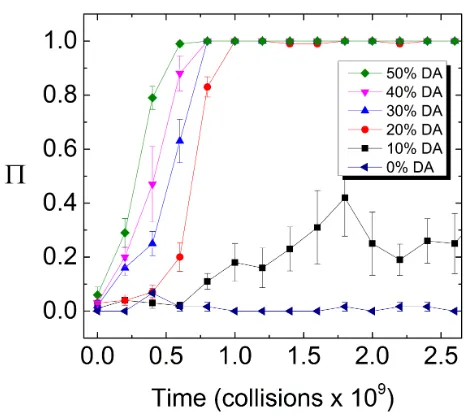
Figure 3.7. Percolation probability of 1.5 wt% chitosan solutions with DA’s ranging from 0% to 50% and a random sequence of GlcNAc monomers ... 108
Figure 3.8. Maximum network size of 1.5 wt% chitosan solutions with DA’s ranging from 0% to 50% and a random sequence of GlcNAc monomers ... 109
Figure 3.9. Percolation probability of chitosan solutions with 30% DA and a random sequence of GlcNAc monomers at concentrations ranging from 0.5 wt% to 2.0 wt% ... 110
Figure 3.10. Number of different inter-chain monomer pairs as a function of the
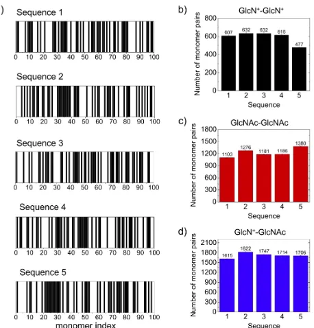
xiv Figure 3.11. a) Monomer sequences used for the 50% DA chitosan systems, b) number
of monomer pairs between two GlcN+
monomers for each monomer
sequence, c) number of monomer pairs between two GlcNAc monomers for each monomer sequence, d) number of monomer pairs between a GlcN+
and GlcNAc monomer for each monomer sequence ... 112
Figure 4.1. Coarse-grained representations for both monomer types. Numbers refer to the coarse-grained site type. ... 148
Figure 4.2. Schematic representations of random, evenly-spaced, and blocky sequences of GlcNAc monomers. Red monomers represent GlcNAc monomers and blue monomers represent GlcN+
monomers. ... 149
Figure 4.3 . Percolation probability for 1.5 wt% chitosan solutions with (a) 10%, (b) 20%, and (c) 30% DA and blocky (blue), random (black), or evenly-spaced (red) sequences of GlcNAc monomers ... 150
Figure 4.4 Snapshots at the end of simulations of 10% (left) and 50% (right) DA chitosan systems at a concentration of 1.5 wt% with a blocky sequence of GlcNAc monomers. The colors of each coarse-grained site correspond to the colors shown in Figure 4.1. ... 151
xv Figure 4.6. Pore size distributions for 1.5 wt% chitosan solutions with DAs ranging
from 10% to 50% and random (black), evenly-spaced (red), and blocky (blue) sequences of GlcNAc monomers ... 153
Figure 4.7. Mean squared displacement of particles with diameters of 20 Å (black) and 60 Å (red) in 1.5 wt% chitosan solutions with DAs of (a) 10% and (b) 50% for a blocky sequence of GlcNAc monomers. Shaded areas represent the error associated with the data. ... 154
Figure 4.8. Number of monomer-monomer associations between a protonated and acetylated monomer (blue), two GlcNAc monomers (red), and two GlcN+
monomers (black) for systems with (a) 10%, (b) 20%, (c) 30%, (d) 40%, and (e) 50% DA and random, even, and blocky sequences of GlcNAc monomers ... 155
Figure 4.9. Average number of monomer associations for each monomer on (a) 10%, (b) 30%, and (c) 50% acetylated chitosan chains with blocky (left) and evenly-spaced (right) sequences of GlcNAc monomers. Black histograms show the monomer sequence, where black segments represent GlcNAc monomers and white segments represent GlcN+
monomers. Red histograms show the average number of monomer-monomer associations for each
monomer on the chain. ... 156
xvi groups: hydroxymethyl (red), protonated amine (blue), ring carbons (cyan), neutral amine (purple), acetyl (green), alkane (yellow). The sites of the coarse-grained HMC are to scale, however this only represents a short
segment of a longer chain. Numbers refer to the coarse-grained type. ... 186
Figure 5.2. Percolation probability over time for 1.5 wt% HMC solutions with
modification densities of (a) 5% and (b) 10% and modification chain lengths of 4 (black), 6 (red), and 8 (blue) spheres ... 187
Figure 5.3. Number of pairs of modification chains that interact for 5% (black) and 10% (red) modified HMC solutions with 4-, 6-, and 8-sphere modification chains ... 188
Figure 5.4. Pore size distributions of systems of (a) 5% and (b) 10% modified HMC with 4- (black), 6- (red), and 8-sphere (blue) modification chains. ... 189
Figure 5.5. Snapshots at the end of simulations of 1.0 wt% HMC with 8-sphere modification chains and (a) 40 Å, (b) 60 Å, and (c) 80 Å diameter
nanoparticles ... 190
Figure 5.6. Percolation probability over time for 5% modified HMC with (a) 4-sphere, (b) 6-sphere, and (c) 8-sphere modification chains with and without 40, 60, and 80 Å diameter hydrophobic nanoparticles ... 191
Figure 5.7. Snapshot of 40 Å nanoparticle (yellow) interacting with 8-sphere
xvii Figure 5.8. Number of modification chains interacting with 40 Å (black), 60 Å (red),
and 80 Å (blue) hydrophobic nanoparticles for systems with (a) 4-sphere, (b) 6-sphere, and (c) 8-sphere modification chains ... 193
Figure 5.9. Number of modification chains interacting with hydrophobic nanoparticles for systems with (a) 40 Å, (b) 60 Å, and (c) 80 Å nanoparticles and
modification chain lengths of 4 (black), 6 (red), and 8 (blue) spheres ... 194
Figure 5.10. Number of pairwise interactions between modification chains for HMC with (a) 4-sphere, (b) 6-sphere, and (c) 8-sphere modification chains in the presence of 40 Å (red), 60 Å (blue), and 80 Å (pink) nanoparticles, and in the absence of nanoparticles (black). ... 195
Figure 6.1 Proposed coarse-grained mapping of tripolyphosphate (TPP) ... 205
1 CHAPTER 1
2
1.1 Motivation
Self-assembled systems have shown promise in applications such as environmental remediation1-4, materials science5-7, and biotechnology8-10. These materials are designed on the molecular level to have a desired functionality, and therefore a controlled assembly in solution. One of the main benefits of self-assembled systems is that structures can be formed on smaller length scales than can be done through traditional manufacturing techniques. These systems can even be designed to respond to stimuli such as changes in pH11,12, temperature13,14, and electric fields15,16. Self-assembled systems based on biocompatible and biodegradable polymers have gained popularity due to their minimal environmental impact and their ability to be used inside the human body. Chitosan is of particular interest because it is both biocompatible and biodegradable, it consists of two monomer types, it is typically charged in solution, and it can be easily modified chemically. For these reasons, chitosan has been used in a wide variety of applications ranging from oil dispersant additives to drug carriers.
3 repulsion between monomers. The acetyl group on the GlcNAc monomers causes hydrophobic and hydrogen bonding interactions between monomers, resulting in net attractive interaction between monomers. Therefore, chitosan solution behavior is controlled by a balance of electrostatic repulsions between GlcN+ monomers and hydrophobic attractions between GlcNAc monomers. Chitosan can also be hydrophobically-modified via a reductive amination reaction of an alkyl aldehyde with the primary amine group of the GlcN monomers. A tool that could quickly investigate various combinations of these parameters would be valuable for designing self-assembled materials based on chitosan. One approach that is often used to gain insight into molecular level behavior is computer simulation.
4 larger systems over longer time scales than can be achieved through traditional all-atom molecular simulations.
Traditional MD simulations are computationally expensive, even when using coarse-grained models19. The interaction potential between two coarse-grained sites is a continuous function of the separation distance between the two sites, e.g. the Lennard-Jones potential. Therefore, the force on each site must be recalculated with every time step to capture the energetics of the system. A small, constant time step is required with a continuous potential because even slight changes in position can result in significant changes to the system energy. If the time step is too large, important dynamic information can be missed, leading to inaccurate results. Therefore, it would be desirable to have a method in which the system can advance through time more quickly, without losing the fundamental behavior of the molecules in the system.
5 the soonest, advances to that time, and analytically updates the collision dynamics. Therefore, the simulation is advanced from collision to collision rather than by a small, constant time step20.
An efficient simulation technique implemented to understand the solution behavior of chitosan as a function of its composition could be used to design materials for a variety of applications. The work in this thesis focuses on development of a novel coarse-grained model of chitosan for use in DMD simulations that can be used to study self-assembly of chitosan in solution.
1.2 Overview
In this section we summarize the remainder of the dissertation. Each chapter contains a literature review and references.
1.2.1 Simulation Study of Hydrophobically-modified Chitosan as an Oil Dispersant Additive
6 chains are more effective at maximizing the oil’s solvent accessible surface area (SASA) than HMCs with 5-sphere modification chains for each of the modification densities tested. Increasing the modification density of HMC with 5-sphere modification chains also increases the surface area of oil over time for each modification density tested. Increasing the modification density of HMCs with 15-sphere modification chains from 4% to 12% results in an increase in the oil’s SASA, however there is negligible change in the oil’s SASA when the modification density is increased from 12% to 20%. This shows that there is a saturation density of long modification chains, above which there is no further improvement in performance. We also show that HMCs with 15-sphere modification chains deform the shape of the oil droplets as a result of the modification chains penetrating deeply into the droplet, while HMCs with 5-sphere modification chains do not significantly change the shape of the oil droplets.
1.2.2 Development of a Coarse-Grained Model of Chitosan for Predicting Solution Behavior
7 potentials were derived using an iterative Boltzmann-inversion technique, and geometric constraints were satisfied based on bond length and angle distributions observed from atomistic simulations. The model was able to closely match chitosan gel formation data as a function of the degree of acetylation (DA). Increasing DA led to a decrease in the time needed to form a percolated network, indicating a decrease in the time needed to form a gel, as was observed experimentally. We also showed that all of the chains in the system assembled into a single network. An analysis of monomer-monomer interactions showed that the interactions between two GlcNAc monomers dominated chitosan self-assembly in solution. Simulations of chitosan under dilute solution conditions showed that our model closely reproduces the radius of gyration (Rg) and persistence lengths (Lp) from several experimental studies.
1.2.3 Effect of Monomer Sequence and Degree of Acetylation on the Self-assembly and Porosity of Chitosan Networks in Solution
8 network later than a blocky sequence, but earlier than an evenly spaced sequence because a random sequence contains both blocky and evenly-spaced regions. We also show that increased blockiness in the sequence of GlcNAc monomers leads to more GlcNAc-GlcNAc and GlcNAc-GlcN+ monomer associations than less blocky sequences. The pore size distributions of networks with different degrees of acetylation (DA) and monomer sequences were also calculated. The results indicate that increasing DA leads to chitosan networks with larger pores because the chains associate more strongly due to the increased hydrophobic interaction between GlcNAc monomers. Blocky sequences of acetylation lead to slightly larger pore size distributions than random and evenly spaced sequences at DA’s below 30%, while all sequences have nearly identical pore size distributions at DA’s above 30%. Finally, we calculated the mean squared displacement of hard-sphere molecules with diameters of 20 Å and 60 Å inside networks consisting of 10% DA and 50% DA chitosan with blocky sequences of GlcNAc monomers. We show that the large pores in a 50% DA network allow equal rates of diffusion of both particles. However, we see that a 10% DA network results in faster diffusion of the 20 Å particle than the 60 Å particle.
1.2.4 Nanoparticle Induced Assembly of Hydrophobically-Modified Chitosan
9 nanoparticles. The results show that 5% modified HMCs only form a stable percolated network in solution with 8-sphere modification chains but not with 4- and 6-sphere modification chains. When the modification density is increased to 10%, stable percolated networks form for HMCs with 6- and 8-sphere modification chains, but not with 4-sphere modification chains. We also see that the pore size distributions of the HMC networks are the same for all modification chain lengths and modification densities, except for 10% modified HMCs with 8-sphere modification chains, which have larger pore sizes due to increased chain hydrophobicity. Next we added 4, 6, and 8 nm diameter hydrophobic nanoparticles at a concentration of 2.0 wt% to HMC solutions of varying modification densities and modification chain lengths at an HMC concentration of 1.0 wt%. Results indicate that the addition of hydrophobic nanoparticles leads to the formation of stable percolated networks while HMCs alone do not. This occurs because the nanoparticles act as junction points that can interact with several HMC molecules at a time. We also see that having a greater number of small nanoparticles leads to the formation of networks earlier in time than having fewer large nanoparticles. The nanoparticles act as association sites that attract several modification chains from different chitosan molecules to a common location.
1.2.5 Future Work
10 parameterizing pH-induced swelling of chitosan hydrogels and parameterizing drug molecules to fit into the framework of our model to study controlled drug delivery using chitosan nanoparticles.
1.3 Publications
Chapters 2-5 are based on the following publications:
Chapter 2: S. W. Benner, V. T. John, and C. K. Hall, “Simulation Study of Hydrophobically Modified Chitosan as an Oil Dispersant Additive”, The Journal of Physical Chemistry B 2015, 119, 6979-6990.
Chapter 3: S. W. Benner and C. K. Hall, “Development of a Coarse-Grained Model of Chitosan for Predicting Solution Behavior”, The Journal of Physical Chemistry B 2016 (in press)
Chapter 4: S. W. Benner and C. K. Hall, “Effect of Monomer Sequence and Degree of Acetylation on the Self-Assembly and Porosity of Chitosan Networks in Solution”,
Macromolecules 2016 (in press)
11
1.4 References
1. Venkataraman P, Tang J, Frenkel E, et al. Attachment of a hydrophobically modified biopolymer at the oil-water interface in the treatment of oil spills. Applied Materials & Interfaces. 2013;5:3572-3580.
2. Jadhav SR, Vemula PK, Kumar R, Raghavan SR, John G. Sugar-derived phase-selective molecular gelators as model solidifiers for oil spills. Angewandte
Chemie-International Edition. 2010;49(42):7695-7698. doi: 10.1002/anie.201002095.
3. Liu G, Yang H, Zhou J. Preparation of magnetic microspheres from water-in-oil emulsion stabilized by block copolymer dispersant. Biomacromolecules.
2005;6(3):1280-1288. doi: 10.1021/bm049318f.
4. Saleh N, Phenrat T, Sirk K, et al. Adsorbed triblock copolymers deliver reactive iron nanoparticles to the oil/water interface. Nano Letters. 2005;5(12):2489-2494. doi: 10.1021/nl0518268.
5. Ikkala O, ten Brinke G. Functional materials based on self-assembly of polymeric supramolecules. Science. 2002;295(5564):2407-2409. doi: 10.1126/science.1067794.
6. Kresge C, Leonowicz M, Roth W, Vartuli J, Beck J. Ordered mesoporous molecular-sieves synthesized by a liquid-crystal template mechanism. Nature.
12 7. Jenekhe S, Chen X. Self-assembly of ordered microporous materials from rod-coil
block copolymers. Science. 1999;283(5400):372-375. doi: 10.1126/science.283.5400.372.
8. Tyrrell ZL, Shen Y, Radosz M. Fabrication of micellar nanoparticles for drug delivery through the self-assembly of block copolymers. Progress in Polymer
Science. 2010;35(9):1128-1143. doi: 10.1016/j.progpolymsci.2010.06.003.
9. Xia X, Wang M, Lin Y, Xu Q, Kaplan DL. Hydrophobic drug-triggered
self-assembly of nanoparticles from silk-elastin-like protein polymers for drug delivery.
Biomacromolecules. 2014;15(3):908-914. doi: 10.1021/bm4017594.
10. Li J, Fan C, Pei H, Shi J, Huang Q. Smart drug delivery nanocarriers with self-assembled DNA nanostructures. Adv Mater. 2013;25(32):4386-4396. doi: 10.1002/adma.201300875.
11. Zhang D, Zhang H, Nie J, Yang J. Synthesis and self-assembly behavior of pH-responsive amphiphilic copolymers containing ketal functional groups. Polym Int. 2010;59(7):967-974. doi: 10.1002/pi.2814.
13 13. Zareie HM, Boyer C, Bulmus V, Nateghi E, Davis TP. Temperature-responsive
self-assembled monolayers of oligo(ethylene glycol): Control of biomolecular recognition. Acs Nano. 2008;2(4):757-765. doi: 10.1021/nn800076h.
14. Pochan D, Schneider J, Kretsinger J, Ozbas B, Rajagopal K, Haines L. Thermally reversible hydrogels via intramolecular folding and consequent self-assembly of a de novo designed peptide. J Am Chem Soc. 2003;125(39):11802-11803. doi:
10.1021/ja0353154.
15. Englander O, Christensen D, Kim J, Lin L, Morris S. Electric-field assisted growth and self-assembly of intrinsic silicon nanowires. Nano Letters. 2005;5(4):705-708. doi: 10.1021/nl050109a.
16. Smith P, Nordquist C, Jackson T, et al. Electric-field assisted assembly and alignment of metallic nanowires. Appl Phys Lett. 2000;77(9):1399-1401. doi:
10.1063/1.1290272.
17. Montembault A, Viton C, Domard A. Rheometric study of the gelation of chitosan in a hydroalcoholic medium. Biomaterials. 2005;26:1633-1643.
18. Montembault A, Viton C, Domard A. Rheometric study of the gelation of chitosan in aqueous solution without cross-linking agent. Biomacromolecules. 2005;6:653-662.
14 20. Smith S, Hall C, Freeman B. Molecular dynamics for polymeric fluids using
discontinuous potentials. J Comput Phys. 1997;134(1):16-30. doi: 10.1006/jcph.1996.5510.
21. Kujawinski EB, Soule MCK, Valentine DL, Boysen AK, Longnecker K, Redmond MC. Fate of dispersants associated with the deepwater horizon oil spill. Environ Sci
Technol. 2011;45(4):1298-1306. doi: 10.1021/es103838p.
22. Piatt J, Lensink C, Butler W, Kendziorek M, Nysewander D. Immediate impact of the exxon valdez oil-spill on marine birds. Auk. 1990;107(2):387-397.
23. Baelum J, Borlin S, Chakraborty R, et al. Deep-sea bacteria enriched by oil and dispersant from the deepwater horizon spill. Environmental Microbiology. 2012;14(9):2405-2416.
24. Thibodeaux LJ, Valsaraj KT, John VT, Papadopoulos KD, Pratt LR, Pesika NS. Marine oil fate: Knowledge gaps, basic research, and development needs; A
perspective based on the deepwater horizon spill. Environ Eng Sci. 2011;28(2):87-93. doi: 10.1089/ees.2010.0276.
25. Zahed M, Aziz H, Isa M, Mohajeri L, Mohajeri S, Kutty S. Kinetic modeling and half life study on bioremediation of crude oil dispersed by corexit 9500. Journal of
15 26. Leahy J, Colwell R. Microbial degradation of hydrocarbons in the environment.
Microbiological Reviews. 1990;54(3):305-315.
27. Rinaudo M. Chitin and chitosan: Properties and applications. Prog Polym Sci. 2006;31(7):603-632. doi: 10.1016/j.progpolymsci.2006.06.001.
28. Majeti NV, Kumar R. A review of chitin and chitosan applications. Reactive &
Functional Polymers. 2000;46:1-27.
29. Aranaz I, Harris R, Heras A. Chitosan amphiphilic derivatives. chemistry and applications. Curr Org Chem. 2010;14(3):308-330.
30. Kumar R, Muzzarelli A, Muzzarelli C, Sashiwa H, Domb AJ. Chitosan chemistry and pharmaceutical perspectives. Chem. Rev. 2004;104(12):6017-6084.
31. Martino A, Sittinger M, Risbud M. Chitosan: A versatile biopolymer for orthapaedic tissue-engineering. Biomaterials. 2005;26:5983-5990.
32. Berger J, Reist M, Mayer JM, Felt O, Gurny R. Structure and interactions in chitosan hydrogels formed by complexation or aggregation for biomedical applications.
European Journal of Pharmaceutics and Biopharmaceutics. 2004;57:35-52.
16 34. Dennis J, Meng Q, Zheng R, et al. Carbon microspheres as network nodes in a novel
biocompatible gel. Soft Matter. 2011;7:4170-4173.
35. Ashmore M, Hearn J, Karpowicz F. Flocculation of latex particles of varying surface charge densities by chitosans. Langmuir. 2001;17(4):1069-1073.
36. Rojas-Reyna R, Schwarz S, Heinrich G, Petzold G, Schütze S, Bohrisch J.
Flocculation efficiency of modified water soluble chitosan versus commonly used commercial polyelectrolytes. Carbohydrate Polymers. 2010;81:317-322.
37. Bratskaya S, Avramenko V, Schwarz S, Philippova I. Enhanced flocculation of oil-in-water emulsions by hydrophobically modified chitosan derivatives. Colloids and
Surfaces A: Physiochemical and Engineering Aspects. 2006;275(1-3):168-176.
38. Lyatskaya Y, Gersappe D, Balazs A. Effect of copolymer architecture on the efficiency of compatibilizers. Macromolecules. 1995;28(18):6278-6283. doi: 10.1021/ma00122a040.
39. Lyatskaya Y, Balazs A. Using copolymer mixtures to compatibilize immiscible homopolymer blends. Macromolecules. 1996;29:7581-7587.
17 41. de Jong J, Subbotin A, ten Brinke G. Spontaneous curvature of comb copolymers
strongly adsorbed at a flat interface: A computer simulation study. Macromolecules. 2005;38(15):6718-6725.
42. Israels R, Foster D, Balazs A. Designing optimal comb copolymers: AC and BC combs at an A/B interface. Macromolecules. 1995;28(1):218-224.
43. Potemkin I, Khokhlov A, et. al. Spontaneous curvature of comblike polymers at a flat interface. Macromolecules. 2004;37(10):3918-3923.
44. Vasilevskaya V, Klochkov A, Khalatur P, Khokhlov A, ten Brinke G. Microphase separation within a CombCopolymer with attractive side chains: A computer simulation study. Macromolecular Theory and Simulations. 2001;10(4):389-394.
45. Malik R, Hall CK, Genzer J. Protein-like copolymers (PLCs) as compatibilizers for homopolymer blends. Macromolecules. 2010;43(11):5149-5157. doi:
10.1021/ma100460y.
46. Malik R, Hall CK, Genzer J. Effect of copolymer compatibilizer sequence on the dynamics of phase separation of immiscible binary homopolymer blends. Soft Matter. 2011;7(22):10620-10630. doi: 10.1039/c1sm06292a.
47. Malik R, Hall CK, Genzer J. Phase separation dynamics for a polymer blend compatibilized by protein-like copolymers: A monte carlo simulation.
18 48. Wang, Z., Hollebone, B.P., Fingas, M., Fieldhouse, B. Sigouin, L., Landriault, M.,
Smith, P., Noonan, J., Thouin, G. Characteristics of spilled oils, fuels, and petroleum products: 1. composition and properties of selected oils. . 2003:1-286.
49. Rapaport DC. Molecular dynamics simulation of polymer chains with excluded volume. J. Phys. A. 1978;11(8):L213-L217.
50. Rapaport DC. Molecular dynamics study of a polymer chain in solution. The Journal
of Chemical Physics. 1979;71(8):3299-3303.
51. Andersen H. Molecular-dynamics simulations at constant pressure and-or temperature. J Chem Phys. 1980;72(4):2384-2393. doi: 10.1063/1.439486.
52. Gaspari G, Rudnick J. The shapes of random walks. Science. 1987;237(4813):384-389.
19 CHAPTER 2
Simulation Study of Hydrophobically-modified Chitosan as an Oil Dispersant Additive
20
Simulation Study of Hydrophobically-modified Chitosan as an
Oil Dispersant Additive
Steven W Bennera, Vijay T Johnb, and Carol K Halla*
aDepartment of Chemical and Biomolecular Engineering, North Carolina State University, 911 Partners Way, Raleigh, North Carolina 27695, United States
bDepartment of Chemical and Biomolecular Engineering, Tulane University, 6823 St. Charles Avenue, New Orleans, Louisiana 70118, United States
Abstract
21 depends on the modification chain length; systems with long modification chains lead to large aspherical aggregates while systems with short modification chains lead to small tightly packed aggregates. A parametric analysis reveals that the most important factor in determining the ability of HMCs to prevent oil aggregation is the interaction between the HMC’s modification chains and the oil molecules, even when using short modification chains. We conclude that HMCs with long modification chains are likely to be more effective at preventing oil aggregation than HMCs with short modification chains, and that long modification chains impede spherical oil droplet formation.
2.1 Introduction
22 consider a viable option for a biocompatible oil dispersant additive, hydrophobically-modified chitosan (HMC), which has been suggested to be both environmentally friendly and effective at preventing oil coalescence.
23 droplets, therefore preventing oil re-coalescence through a combination of electrostatic and steric repulsion1.
24 density44. Other simulation studies have analyzed the orientation of copolymers at the interface between two immiscible phases and their ability to prevent phase separation45-47, but focused mainly on linear copolymers.
The goal of our research is to understand how the architecture of an HMC affects its ability to prevent oil aggregation with a view towards using HMCs for oil spill remediation. Simulations provide us with a molecular-level perspective on the interaction between HMCs and oil that cannot be obtained through experiment alone. Although the experimental work of Venkataraman and coworkers on HMCs has given good insight into the ability of HMCs to prevent oil coalescence, a number of questions remain such as the following. How does the length of the hydrophobic modification chains or the number of modification chains along the chitosan backbone (modification density) affect the efficacy of HMCs as oil stabilizers? What concentration of HMCs is necessary for oil droplet stabilization? What are the mechanisms by which HMCs stabilize oil droplets and how are they affected by the HMC architecture? What role does the chitosan backbone play in preventing oil droplets from aggregating? Answering these questions could lead to optimum HMC architectures for different types of oil spills and lower demand for oil dispersants.
25 chains. Both the oil and chitosan molecules consist of chains of well and square-shoulder spheres. Water is modeled implicitly in all simulations, making the square-well and square-shoulder interactions potentials of mean force. Simulations are performed at various values of the modification chain length, modification density (percentage of chitosan backbone spheres containing modification chains), and overall HMC concentration. To determine how these parameters affect the HMCs ability to prevent oil aggregation, and the mechanism by which this is effected, we monitor the oil’s solvent accessible surface area (SASA), and the number, size, and shape of oil aggregates over the course of the simulations. The oil’s SASA gives a measure of how much oil surface area would be exposed to ocean bacteria leading to natural degradation. The oil aggregate size distribution indicates if the HMCs are preventing the oil from coalescing, therefore acting as an effective stabilizer. The shape of the oil aggregates is determined by calculating their asphericity, where the more aspherical the oil aggregates become, the more surface area is exposed to bacteria.
26 with many short modification chains, even with the same total number of modification spheres. Finally, analysis of the contributions of the interaction energies between different types of spheres showed that the attractive interaction between the modification chains and the oil chains was the dominant interaction governing the HMC behavior, and that excluded volume interactions were not important in determining the effectiveness of HMCs even at high HMC volume fractions.
2.2 Methods
27 containing modification chains, was 4%, 12%, or 20%. Diagrams illustrating the architecture of the HMCs used in the simulations can be seen in Figure 2.1. The sphere diameter, σ, for all species in the system is 1.0, and the bond length between adjacent spheres on the same chain is allowed to fluctuate between σ(1+δ) and σ(1-δ), where δ = 0.01, making the spheres tangent. If adjacent spheres reach the maximum or minimum bond length, they hit an infinite repulsive potential that bumps them back to within the allowed bond distance49,50. Stiffness is incorporated into these chains using “pseudobonds” in which the minimum and maximum angles that can form between next nearest neighboring spheres along the chain are set to 122 and 180 degrees respectively for the chitosan backbone, and 90 and 180 degrees respectively for the modification and oil chains. The chitosan backbone is stiffer than that of the alkane chains for two reasons: 1) to emulate the rigidity of a chitosan molecule, and 2) to mimic the electrostatic repulsion that occurs between the cationic chitosan monomers in slightly acidic conditions. The stiffness of the oil and modification chains is maintained by a set of pseudobonds to mimic the stiffness of real alkane chains, and to prevent the oil and modification chains from collapsing in an unrealistic manner.
Interactions between spheres are modeled using square-well or square-shoulder potentials depending on whether the interaction is attractive or repulsive. The potential energy between spheres of type i and j, Uij(r), as a function of distance between the spheres, r, is given by the following potentials:
𝑈!"(𝑟) =
∞𝑖𝑓 𝑟 ≤ 𝜎
𝜖!" 𝑖𝑓𝜎< 𝑟≤ 𝜆𝜎
0𝑖𝑓 𝑟> 𝜆𝜎
28 where 𝜖!" is the interaction energy between spheres i and j, and the well or square-shoulder width is taken to be λσ = 1.75. Table 1 lists the interaction energies between each type of sphere in the system. Negative values of the interaction energy represent attractions and positive values represent repulsions. The energies were chosen to mimic the types of interactions expected in a system of polar and non-polar molecules in water. Water is modeled implicitly in all simulations, making interaction energies between all spheres potentials of mean force in water. Chitosan, being polar, preferably interacts with itself over hydrocarbons. Therefore, the chitosan spheres are attracted to each other, but repelled by all other spheres in the system. The hydrophobic modification chains and the oil molecules represent alkanes, and therefore are attracted to each other and repelled by chitosan. The strength of attraction between chitosan spheres is half that of the attractive interactions between hydrophobic groups to help keep the chitosan backbone extended, as it would be in the presence of water molecules. The attractive energy between chitosan monomers is weaker than the attractive energy between modification spheres, and between oil spheres, so as to prevent the chitosan backbone from collapsing on itself, but is strong enough to encourage association with other chitosan molecules.
Details of the simulation conditions are the following. The packing fraction, η =
29 = 0.5 contain approximately 6000 HMC spheres and 6000 oil spheres, systems with ϕhmc = 0.35 contain approximately 4200 HMC spheres and 7800 oil spheres, and systems with ϕhmc = 0.2 contain approximately 2400 HMC spheres and 9600 oil spheres.
DMD simulations were used in place of traditional molecular dynamics (MD) to increase the speed of the simulations while still capturing the fundamental behavior of the system19. Unlike traditional MD simulations, which numerically solve Newton’s equations of motion every time step, DMD is an event driven technique20. The DMD simulation algorithm searches for the soonest-to-occur event (collision between spheres), advances the time to the point that the collision occurs, and analytically calculates the new particle positions and velocities after the collision20. An event occurs any time a particle reaches a discontinuity in the interaction potential as a function of separation distance such as at the boundary of a hard sphere, square-well, or square-shoulder potential. Because the method is event driven, a collision occurs every time step, avoiding the need to re-calculate collision dynamics multiple times before particles are within the interaction distance of each other. Following a collision, the particles in the simulation move linearly until their next collision occurs.
31 the formation of different equilibrium structures because oil aggregation would have already begun by the time HMCs were added. We plan to investigate this phenomenon in future work to determine how the addition of HMCs at different times affects the system equilibrium, giving insight into the importance of response time to HMC efficacy.
32 Second, we calculated the percent increase in oil SASA for various HMC architectures over systems without HMCs present. The percent increase in the oil SASA is given by:
%𝑖𝑛𝑐𝑟𝑒𝑎𝑠𝑒 𝑖𝑛 𝑜𝑖𝑙 𝑆𝐴𝑆𝐴= !"!"!"#!!"!"!"#$%
!"!"!"#$% × 100 (2.2)
where SASAHMC is the oil SASA with HMCs present and SASAnoHMC is the oil SASA without HMCs present. The number and size of the oil aggregates was also calculated at various time points to determine if the HMCs could prevent aggregation and to give insight into the mechanism of aggregation. These quantities measure how effectively the HMCs prevent oil aggregates from coalescing over time.
Third, we analyzed the shape of the oil aggregates to determine how the HMC architecture affected the ability of oil to form small droplets. The aggregate shape was characterized in terms of its asphericity. 52,53 This method involves calculating the principal components of the gyration tensor, S, for each oil aggregate:
𝑺= ! !
𝑥!−𝑥!" !
! !(𝑥!−𝑥!")(𝑦!−𝑦!") !(𝑥!−𝑥!")(𝑧!−𝑧!")
(𝑥!−𝑥!")(𝑦!−𝑦!")
! ! 𝑦!−𝑦!" ! !(𝑦!−𝑦!")(𝑧!−𝑧!")
(𝑥!−𝑥!")(𝑧!−𝑧!")
! !(𝑦!−𝑦!")(𝑧!−𝑧!") ! 𝑧!−𝑧!" !
(2.3)
where xi, yi, and zi are the coordinates of each oil sphere, i, in the aggregate, xcm, ycm, and zcm are the coordinates of the aggregate’s center of mass, and N is the total number of oil spheres in the aggregate. The eigenvalues of the gyration tensor λ1, λ2, and λ3, are the principal components of the radius of gyration, Rg, defined by:
𝑅!! = 𝜆
33 where λ1, λ2, and λ3 are the eigenvalues of the gyration tensor. These principal components are then used to calculated the oil aggregate asphericity, A, defined as:
𝐴= !!!!! !!!!!!! !!!!!!! !
! !!!!!!!! ! (2.5)
where λ1 ≥ λ2 ≥ λ3. The asphericity has a minimum value of 0 for a perfectly spherical aggregates and a maximum value of 1 for completely linear aggregates. The radius of gyration and asphericity data were averaged over the final 100 million collisions of the simulations (with data recorded every 10 million collisions) and over 5 simulation replicates. All of the previously mentioned analysis techniques were performed on oil aggregates in systems with and without HMCs to determine the impact of HMCs on oil aggregation. Error bars for all quantities calculated represent the standard deviation from the average of each data point over 3 to 5 replicates.
2.3 Results
34 end of the simulations (2 billion collisions), the oil-only system formed a single large aggregate as can be seen in Figure 2.1 (e). Note that although there appear to be four separate aggregates in Figure 2.1(e), there is actually only one aggregate, which crosses the periodic boundary conditions. In contrast, the oil + HMC system formed many smaller oil aggregates, which can be seen in Figure 2.1(f). We speculate that the HMCs help stabilize the smaller oil aggregates and prevent them from coalescing via the modification chains anchoring into the oil droplets and the chitosan backbone remaining on the perimeter of each droplet. We believe that a combination of repulsion between the chitosan and oil spheres and steric hindrance of the chitosan backbone covering the oil aggregates prevents the oil from coalescing as much as in systems without HMCs. Once the modification chains of the HMCs penetrate the oil aggregates, the motion of the chitosan backbone is restricted because it is pinned to the oil aggregates at multiple locations. Therefore, the backbone acts to block new oil chains from joining the aggregate.
36 Figure 2.4 summarizes the efficacy of different HMC architectures at concentrations,
ϕhmc = 0.5, 0.35, and 0.2, by plotting the percent increase in oil SASA resulting from (a)
5-sphere and (b) 15-5-sphere modification chain HMCs over the oil SASA without HMCs present at the end of the simulations at various modification densities. Figure 2.4 confirms that there is a relatively linear trend in the percent increase in oil SASA with increasing modification density for HMCs with 5-sphere modification chains. In contrast, as we saw from Figure 2.3, there is clearly a modification density of HMCs with 15-sphere modification chains, above which the percent increase in oil surface area remains essentially unchanged, even at the lowest HMC concentration tested (ϕhmc = 0.2). This shows that the saturation phenomenon persists regardless of the HMC concentration, and we can therefore conclude that it is unnecessary to use a modification density above 12% for HMCs with 15-sphere modification chains at any HMC concentration. To determine the optimum modification density with 5-sphere modification chains, we would need to increase the modification density further, however this would far exceed the modification densities used in experiments.
37 compares the oil aggregate size distributions for simulations of 20% modified HMCs with 5 or 15-sphere modification chains at ϕhmc = 0.5 at various times throughout the simulation. The number of small aggregates (50 chains or less) significantly decreases over time as the aggregates coalesce. This behavior reflects what happens in an oil spill scenario, where small oil droplets coalesce into a slick on the ocean surface. Figure 2.5 also shows that the aggregate size distributions using 5 or 15-sphere modification chains differ significantly for 20% modified HMCs. There are nearly twice as many small oil aggregates (50 chains or less) for HMCs with 5-sphere modification chains as there are for 15-sphere modification chains after 1.25 billion collisions. By the end of the simulations, the aggregate size distribution is skewed to favor smaller aggregates for 5-sphere modification chains, but is more evenly distributed for 15-sphere modification chains. Therefore, at this high modification density, HMCs with short modification chains result in many small aggregates while HMCs with long modification chains result in a few large oil aggregates.
38 HMCs with short or long modification chains because there were too few HMCs to make a significant impact on the oil aggregate size distribution. However, even low concentrations of HMCs lead to more small aggregates than systems without HMCs, which form a single large aggregate by the end of the simulations. Therefore, the HMCs are beneficial in reducing oil aggregation even at the lowest concentrations tested.
39 direction going into the page. The asymmetry in oil aggregate shape is most noticeable at high modification densities, because there are more modification chains present to penetrate each oil droplet. Figure 2.7(c) reveals many pores in the oil aggregates, providing visual evidence of the ability of long modification chains to penetrate into the aggregates. In contrast, very few pores are visible in the oil aggregates in Figure 2.7(b), showing the inability of the short modification chains to penetrate deeply into the oil aggregates. We would like to clarify that the pores observed in Figure 2.7(c) are merely the voids left by removing the HMCs from the snapshot. Their presence demonstrates how effectively the long modification chains penetrate the oil aggregates.
40 resulting in the minimum possible surface area. Therefore, even though there are a greater number of small aggregates with 5-sphere modification chains, all of the aggregates minimize their surface area by taking on a spherical shape. Although there are fewer (and larger) aggregates in systems with 15-sphere modification chains, the HMCs more effectively penetrate into the oil aggregates, elongating the aggregates, and creating more oil surface area.
41 modification spheres and oil spheres, while the bottom snapshot (5-sphere modification chains) shows separate oil and modification domains with no significant penetration of the modification chains into the oil aggregates. The percentage of modification spheres interacting with oil spheres is nearly identical regardless of modification density (data not shown).
42 At this point the effectiveness of HMCs as oil stabilizers has been analyzed using a number of techniques, however one important question remains. Are HMCs with few long modification chains better at preventing oil aggregation than HMCs with many short modification chains if the total number of modification spheres is the same? To determine if the architecture plays a role in oil stabilization, it is necessary to compare two different HMC architectures with the same total number of chitosan and modification spheres per molecule. This determines if stabilizing oil droplets depends on more than just the total number of modification spheres in the system. Therefore we compared simulations of 4% modified HMCs with 15-sphere modification chains and 12% modified HMCs with 5-sphere modification chains in oil at ϕhmc = 0.5. The HMCs that were 4% modified with 15-sphere modification chains had two modification chains on the chitosan backbone, while the HMCs that were 12% modified with 5-sphere modification chains had six modification chains on the chitosan backbone. However, both HMCs had the same total number of chitosan spheres (50) and modification spheres (30) per molecule. The final oil SASA using HMCs with 15-sphere modification chains was 12% higher than the oil SASA using HMCs with 5-15-sphere modification chains (data not shown). This is consistent with the behavior discussed previously where longer modification chains led to a larger oil SASA, and also shows that the HMC architecture does play a role in oil dispersion, even for HMCs with the same number of modification spheres.
43 chains) than HMCs with short modification chains even though the total number of spheres for the two HMCs is the same. We also observed the formation of slightly more large aggregates (>200 chains) with long modification chain HMCs than with short modification chain HMCs. These results are in agreement with the previously mentioned aggregate size distributions, where long modification chains promoted the formation of larger oil aggregates. From these results we can conclude that HMC architecture does affect both the oil SASA and the size distribution of oil aggregates, and that the HMC efficacy is dependent on more than just the total number of modification spheres in the system.
To ensure that the increase of oil SASA in systems containing HMCs was not simply due to the HMCs “getting in the way” of the oil chains, the interaction energies between the various species were systematically set to zero one at a time, to pinpoint the important interactions. The rationale for this exercise is that if the HMCs simply prevented oil aggregation because they took up space in the simulation box, setting attractive/repulsive interactions between HMCs and oil to zero would result in approximately the same oil SASA over time as simulations with all of the interactions accounted for between the HMCs and oil. Note that the attractive interaction between oil spheres is always present to ensure that the oil aggregates in all simulations. Four total cases were tested to determine the most important interaction energies: (1) no interactions were set to zero, (2) chitosan backbone interactions were set to zero, (3) modification chain interactions were set to zero, (4) all interaction energies were set to zero.
45
2.4 Discussion and Conclusions
46 Next we looked at the oil aggregate size distributions for systems of HMCs with various modification densities and modification chain lengths. This analysis revealed that HMCs with long modification chains led to fewer and larger oil aggregates than systems with short modification chains. This contradicted the results we expected, given that HMCs with long modification chains had larger oil SASAs than HMCs with short modification chains. One would have expected that an increase in oil SASA would coincide with a greater number of small oil aggregates rather than fewer large oil aggregates. The only way it would have been possible to have a larger oil surface area and larger oil aggregates would be for the aggregates to be stretched. To test this hypothesis we first looked at snapshots of the oil phase at the end of simulations to get a qualitative understanding of the oil aggregate shape. It was clear from these snapshots that the oil aggregates in systems of HMCs with long modifications were indeed more stretched and aspherical than oil aggregates in a system with short modification chain HMCs. We concluded that the oil aggregate asphericity for HMCs with 5-sphere modification chains does not vary significantly with increasing modification density, while that for 15-sphere modification chains increases by approximately 50% going from the lowest to highest modification densities. The longer modification chains more effectively penetrate into the oil aggregates, deforming their shape.
47 aggregates, in turn restricting the movement of the aggregates and preventing aggregation. In contrast, we have shown that the long modification chain HMCs prevent aggregation by penetrating deeply into the aggregates and preventing them from forming small, spherical droplets.
In conclusion we have gained insight into the optimum HMC architectures for preventing oil aggregation. Our results conceptually agree with the experimental work of Venkataraman and coworkers1 and can be used to help design effective HMC oil stabilizers. One way that our simulations differ from the work of Venkataraman and coworkers is that we did not include Corexit in the system. Corexit is primarily used to break up oil into smaller droplets. In a way we accounted implicitly for addition of Corexit by starting our simulations in a random initial configuration with oil molecules already broken up. If we were to include Corexit in the simulations, the efficacy of HMCs might increase due to electrostatic attraction between the cationic chitosan monomers and the anionic surfactant, dioctyl sodium sulfosuccinate (DOSS), present in Corexit. This might allow the HMCs to adhere more strongly to the oil droplets and possibly travel to the oil/water interface more quickly. We plan to include Corexit in a follow-up study. In its current state our model can be easily applied to study different chitosan molecular weights, different types of modification chains, and different HMC concentrations. We are currently extending our model to include more details about the chitosan backbone such as the degree of acetylation and surface charge, making the model more universally applicable to a variety of conditions.
48 used an implicit solvent approach, which does not accurately represent the diffusion of molecules or hydrodynamics. Because there are no water molecules to collide with the solute, the solute molecules travel more quickly through the simulation box than they would in the presence of water. The second limitation is that it is difficult to make a direct correlation between the reduced temperature in the simulation and real temperature. Values of the reduced temperature and interaction energies were chosen to make the oil aggregate gradually over the course of the simulation (several hundred million collisions) as opposed to being derived via multi-scale modeling of atomistic simulations. Therefore the chosen temperature is not directly related to the real temperature, as would be the case in atomistic simulations. The third limitation of this method is that we do not have a way to correlate simulation time to real time because molecules move in a straight line in a vacuum between collisions, rather than traveling through solvent. In order correlate our results to a real time scale we would have to compare the time it takes for a specific molecular mechanism to occur in experiments and simulations. Unfortunately we are unable to identify a mechanism that would be distinguishable in both experiments and simulations to compare the time scales.
2.5 Acknowledgements
49
2.6 References
1. Kujawinski EB, Soule MCK, Valentine DL, Boysen AK, Longnecker K, Redmond MC. Fate of dispersants associated with the deepwater horizon oil spill. Environ Sci
Technol. 2011;45(4):1298-1306. doi: 10.1021/es103838p.
2. Piatt J, Lensink C, Butler W, Kendziorek M, Nysewander D. Immediate impact of the exxon valdez oil-spill on marine birds. Auk. 1990;107(2):387-397.
3. Baelum J, Borlin S, Chakraborty R, et al. Deep-sea bacteria enriched by oil and dispersant from the deepwater horizon spill. Environmental Microbiology. 2012;14(9):2405-2416.
4. Thibodeaux LJ, Valsaraj KT, John VT, Papadopoulos KD, Pratt LR, Pesika NS. Marine oil fate: Knowledge gaps, basic research, and development needs; A perspective based on the deepwater horizon spill. Environ Eng Sci. 2011;28(2):87-93. doi: 10.1089/ees.2010.0276.
5. Zahed M, Aziz H, Isa M, Mohajeri L, Mohajeri S, Kutty S. Kinetic modeling and half life study on bioremediation of crude oil dispersed by corexit 9500. Journal of
Hazardous Materials. 2011;185:1027-1031.
6. Leahy J, Colwell R. Microbial degradation of hydrocarbons in the environment.
Microbiological Reviews. 1990;54(3):305-315.