Development and Optimization of an Alternative Electrospinning Process for High Throughput

ABSTRACT

THOPPEY MUTHURAMAN, NAGARAJAN. Development and Optimization of an

Alternative Electrospinning Process for High Throughput. (Under the direction of Dr. Russell E. Gorga and Dr. Laura I. Clarke).

Development and Optimization of an Alternative Electrospinning Process for High Throughput

by

Nagarajan Thoppey Muthuraman

A thesis submitted to the Graduate Faculty of North Carolina State University

in partial fulfillment of the requirements for the degree of

Master of Science

Textile Engineering

Raleigh, North Carolina 2010

APPROVED BY:

_______________________________ ______________________________ Dr. Russell E. Gorga Dr. Laura I. Clarke Committee Chair Co – Chair

________________________________ ______________________________

Dr. Maury Balik Dr. Jason Bochinski

DEDICATION

BIOGRAPHY

Nagarajan Thoppey Muthuraman was born on July 12th, 1978 in the city of Madurai, India. He obtained his Diploma in Textile Technology in 1996 from the State Board of Technical Education in Chennai, India. He worked as a production executive in Coats India Limited, a spun-yarn manufacturing company in Tuticorin, India for four years. He obtained a Bachelors of Textile Technology in 2004 from University of Madras, Chennai, India in the following three years. After his graduation, he worked as a compliance auditor and product development assistant for Epic Designers Private Limited, an apparel manufacturer in Dhaka, Bangladesh for two and a half years.

ACKNOWLEDGEMENTS

I would like to express my sincere gratitude to Dr. Russell E. Gorga and Dr. Laura I. Clarke for their constant support and encouragement during this research work. Dr. Gorga has been an incredible mentor and great source of inspiration. He has been always there to point out the right direction, whenever and wherever I needed. I would like to thank Dr. Jason Bochinski for his valuable guidance in this research. I am indebted to Dr. Clarke and Dr. Bochinski for nurturing and developing the scientist within me. It has been a wonderful experience to learn from all of them. I take this opportunity to thank all of their support and patience especially in the process of documenting this work. I also thank Dr. Maury Balik for agreeing to be in the committee as a minor representative.

I submit my sincere thanks and appreciation to Mr. Hai Bui and Mr. Dzung Nguyen (Win) for their daily assistance. I acknowledge all my lab mates especially Beth, Kelly, Erik, Remya, Rebecca and Mary for their help and fruitful discussions. I am thankful to Mr. Chuck Mooney (AIF) and Mrs. Judy Elson for training me on the Scanning Electron Microscope. I would like to thank Ms. Angie Brantley for her help and coordination from day one.

Life here in the United States would not have been so enjoyable or cheerful without great people around me. I feel immense pleasure to acknowledge and thank all of them especially Mridula, Vamsi, Anjali, Anita, and my aunt and cousins. I would be remiss if I did not acknowledging Krishna Bala for her unconditional love and support in making this journey so cheerful and meaningful.

TABLE OF CONTENTS

LIST OF FIGURES ... viii

LIST OF TABLES ... xi

CHAPTER 1 INTRODUCTION ... 1

CHAPTER 2 BACKGROUND ... 7

2. 1 Introduction ... 7 

2. 2 Historical overview ... 7 

2. 3 Apparatus ... 8 

2. 4 Physical description of the electrospinning process ... 11 

2.4.1 Taylor cone ... 12 

2.4.2 Linear region ... 14 

2.4.3 Whipping region ... 15

2. 5 Electrospinning variables ... 17 

2.5.1 Material variables ... 19 

2.5.1.1 Polymer concentration and molecular weight ... 19 

2.5.1.2 Solution conductivity ... 19 

2.5.1.3 Surface tension ... 20 

2.5.1.4 Other material variables ... 20

2.5.2 Process variables ... 20 

2.5.2.1 Applied voltage - Magnitude ... 20 

2.5.2.2 Applied voltage - Signal and Polarity ... 22 

2.5.2.3 Volume feed rate ... 23 

2.5.2.4 Working distance ... 23 

2.5.2.5 Other process variables ... 24 

2.5.3 Equipment variables ... 24 

2.6 Scale up approaches ... 25 

2.6.1 Confined fluid flow ... 26 

2.6.2 Unconfined fluid flow ... 27 

2.7 Self-Assembled Monolayer (SAM) ... 29 

2.8 Electric field simulations ... 31 

CHAPTER 3 RESEARCH OBJECTIVES ………..………. 33

CHAPTER 4 EXPERIMENTAL ………..……… 35 

4.1 Materials ... 35 

4.2 Apparatus ... 37 

4.3 Fiber characterization ... 40 

CHAPTER 5 RESULTS AND DISCUSSION ……… 42

5.1 Electric field simulations ... 42 

5.2 Jet formation ... 45 

5.3 Jet profiles ... 50 

5.4 Processing parameters-fiber properties relationships ... 54 

5.4.1 Fiber diameter and diameter distribution ... 54 

5.4.1.1 Effect of fluid flow... 54 

5.4.1.2 Effect of applied voltage and working distance ... 56 

5.4.2 Spinnability and Porosity ... 57 

5.4.3 Effect of multiple feed streams on morphology and production rate ... 58

5.5 Spinning from multiple plates ... 60 

      5.5.1 Electric field Simulation ……...60 

5.5.2 Experimental observations ... 61 

5.5.3 Intermittent spinning in TNE ... 62 

5.5.4 Fabrication rate ... 62 

5.6 Spinning from edge-cylinder ... 63 

5.6.1 Experimental ... 63 

5.6.2 Electric field simulation ... 64 

5.6.3 Preliminary results ... 64 

CHAPTER 6 CONCLUSIONS...67

CHAPTER 7 FUTURE WORK...69

REFERENCES...70

LIST OF FIGURES

Figure 1.1: Potential applications of nanofibers………3

Figure 2.1: Schematic diagram of traditional needle electrospinning (TNE)....………..9

Figure 2.2: Schematic of a droplet from a single needle in an applied electric field...………13

Figure 2.3: Illustration of Earnshaw instability, leading to bending of an electrified jet…....18

Figure 2.4: Representation of multiple instabilities from a single jet ……….….18

Figure 2.5: Classification of electrospinning variables………...21

Figure 2.6: Processing map – effect of process variable on fiber diameter………….………24

Figure 2.7: Classification of scale-up approaches………..28

Figure 2.8: Formation of SAM on a silica surface using decyltrichlorosilane ……..….……30

Figure 2.9: Representation of water contact angle (θ) of a substrate

a) before SAM and b) after SAM ………...30

Figure 4.1: Contact angle measurements for an aluminum plate whose wettability has been chemically modified by treatment with

decyltrichlorosilane (C10) for a) water (105 ± 3˚) and b) 6 wt % PEO +

water spinning solution (87 ± 3˚)………...……… 36

Figure 4.3: (a) Illustration of single edge plate electrospinning, θ and

direction of gravity (Fg), and (b) Multi-plate electrospinning ‘waterfall”)………….…...38

Figure 5.1: Electric field distributions for TNE geometry with 15 cm

working distance and 15 kV ………...……43

Figure 5.2: Electric field distributions for parallel plate geometry

with 15 cm working distance and 15 kV………..………...43

Figure 5.3: Electric field distributions for edge-plate geometry

with 15 cm working distance and 15 kV………….……….…...44

Figure 5.4: PEO-polymer solution droplet (doped with R6G) falling from the plate and subsequent jet initiation process. Sequential video images taken under room light

illumination . Arrows in the images (d,e,f) shows the jet direction……….……48

Figure 5.5: Average fiber diameter and jet linear region length vs. feed rate in (a) TNE process with 15 cm working distance and 11 kV (b) TNE and

Edge plate electrospinning process with 35 cm working distance and 28 kV…………...…..52

Figure 5.6: (a) Schematic representation of jet in plate electrospinning (b) Image of

jet profile at 35 cm working distance ………..53

Figure 5.7: Amplitude A of whipping instability as measured from the radius of the instability envelope vs. axial distance from the onset of whipping instability fit to an exponential function. Shin‘s whipping trend is shown with a

dotted line in conjunction with the primary and secondary cones observed in

TNE and edge- plate electrospinning for this work ………....53

Figure 5.8: Comparison of electrospun nanofibers from (a) TNE geometry at 15 cm working distance and 11 kV (b) edge-plate geometry at 35 cm working distance

and 28 kV………...55

Figure 5.10: (a) Electric field distributions of edge cylinder geometry (b) magnified image of the edge (arrow indicates the direction of the jet)………...……...……...……...65

Figure 5.11: SEM image of edge-cylinder electrospun nanofibers (at 14 cm working

LIST OF TABLES

Table 1.1: Comparison of processing techniques for obtaining nanofibers ……….2

Table 5.1: Electric field strength and jet profiles measurements of TNE and

Edge-plate electrospinning process..………50

Table 5.2: Effect of multiple spinning sites (pipettes) on average fiber diameter

And fabrication rate ………58

Chapter 1

Introduction

Of all the techniques, electrospinning is the most common and a relatively simple technique for nanofiber fabrication [1-6]. Nanofibers with diameters of 40 – 1000 nm can be produced from polymer solutions or melts and collected as nonwoven mats with ~70-80% porosity. With small modifications to the electrospinning apparatus, fibers with uni-axial arrangement can be obtained.

Electrospun nanofibers have significant technological promise due to their high surface area to volume ratio and the resultant nanofibrous mats are lightweight due to their high porosity. Figure 1.1 shows many potential applications of polymeric nanofibers. The high relative surface area has the potential to facilitate catalysis and other sensitive surface reactions or to enable highly sensitive sensors [1]. For example, humidity sensors based on a

                        Process Current use (level of technology) Can the process be scaled?

Repeatability Convenient to process?

Control of Dimension

Drawing Laboratory No Yes Yes No

Template

Synthesis Laboratory No Yes Yes Yes

Phase

Separation Laboratory No Yes Yes No

Self-Assembly Laboratory No Yes No No

Electrospinning

Laboratory (with potential

for industrial processing)

Yes Yes Yes Yes

PEO nanofiber carrying 1 wt% of LiClO4 showed a sensitivity level six times that of comparable thin-film material [7]. Nanofibrous materials doped with conductive particles have shown excellent conductivity [8]. Such materials are well suited for conductive sensor applications. If the nanofibrous material (doped with a conductive particle) were to come in contact with a chemical and/or biological agent that could swell the fiber, the volume of the material would increase (due to the swelling) which in turn would disrupt the connectivity of the conductive particle. This, in turn, could alter the nanofibrous mat’s electrical resistance. Although this phenomenon is already utilized in electronic-nose technology using polymer films [9], nanofibrous mats are efficient because of their high specific surface area.

The nanofiber diameter and porosity are well-suited for medical applications such as tissue scaffolds, drug delivery devices, and wound protection [4, 10]. The success of polymer nanofibrous mats in tissue scaffold applications occurs primarily because the fiber diameters and overall porosity (and pore size) are on the same scale as the structural features present in body tissue environments (i.e. the extracellular matrix). The ultimate goal will be to seed nanofibrous scaffolds with cells that can grow and differentiate in vitro or in vivo to replace damaged tissue. Bio-degradable polymer nanofibers play an important role in such applications.

In addition, nanofibrous scaffolds doped with conductive particles have been shown to perform as strain sensors (functioning much like the conductive sensors described above) [12]. Other important potential applications of nanofibers with conductive particles include intelligent and communicative textile structures, smart analyte vapor sensors for defense and security applications, environmental and medical diagnostics, self-reporting smart structures, and, in particular, self-reporting filtration media.

those from the more traditional (i.e., aperture-based) approaches. Thus, in aperture-free systems, with increased throughput the preferred fiber morphology may be compromised.

Chapter 2 Background

2.1 Introduction

This chapter will provide a comprehensive overview of fundamentals of the electrospinning process and other elements that will be introduced in the later chapters. Section 2.2 provides a historical overview of electrospinning while section 2.3 focuses on the apparatus. Section 2.4 outlines various variables involved in the electrospinning process. Section 2.5 reviews the approaches so far attempted in scaling up the process. Finally, sections 2.6 and 2.7 provide an overview of self-assembled monolayers and electrostatic simulation respectively.

2.2 Historical overview

Baumgarten (1971) [19] reported comprehensive experiments on the electrostatic spinning of acrylic microfibers from solution, and published many state-of-the-art stop-motion photographs of electrospinning jets. A decade later Larrondo and Manley [20] published their works on electrospinning from polymer melts. A large break in the progress of research from 1944 to 1971 is believed to be due to the absence of industrial initiatives or applications for such nanofibrous materials. Applications of electrospun nanofibers became apparent when Donaldson Co., Inc., (USA) introduced their first commercial product (filters) in 1981 and a widespread interest was created across many research fields. (It is germane to note, however, that it is also reported [21] that a team in the USSR (Rosenblum and Petrianov-Sokolov) helped establishing the first known industrial facility for producing fibrous materials for military gas masks.) More recently, research on the process of electrospinning received a great deal of academic attention over the last decade, once Reneker and coworkers [22-24] spun various kinds of polymers and characterized their properties. Since then, the number of research publications has grown exponentially in the past 15 years and continues to do so.

2.3 Apparatus

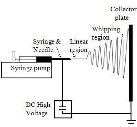
Figure 2.1 Schematic diagram of traditional needle electrospinning (TNE)

Numerous modifications in the TNE set-up have been investigated in order to achieve (or attempt to achieve) enhanced properties and collection methods of nanofibers. These modifications are discussed below by classifying the basic set-up in to three zones, namely: i) the feed zone; ii) the spinning zone; and, iii) the collection zone.

i) Feed zone (from the reservoir to the needle tip in TNE): The aim of the feed zone is to continuously provide a fluid that results in the formation of a fine, electrically charged droplet (upon applying electric field) for the electrospinning process. Modifications in the feed zone include different needle designs (single and bicomponent needles [25, 26], multiple needles (discussed in 2.7)), different electrode designs (needle with flat plate or cylindrical electrodes [27, 28]), and the addition of external systems like an air-blower that assists in the evaporation process [29]. These modifications help in altering the morphology (and, in some cases, the throughput) of the final fiber collected in the collection zone.

iii) Collection zone (collector surface): The object of this zone is to gather nanofibers from the spinning zone by providing a suitable (usually grounded) potential surface. A number of modifications [32-34] in this zone have been explored in order to obtain different structures (such as yarns, mats, wound filaments, or conduits) or different alignments of the fibers in a plane (such as random, parallel, or pseudo-woven).

All these modifications are designed to obtain different forms of nanofibrous materials or different morphologies while the overall electrospinning process remains the same. A detailed description of fundamental physics behind the electrospinning process is discussed in the following section.

2.4 Physical description of the electrospinning process

finally leaving dried nanofibers on the collector. The physical characteristics of the electrospinning process can be described by these three regions, namely, the Taylor cone, the linear region, and the whipping region [23, 36].

2.4.1 Taylor cone

In 1969, Taylor studied the deformation of liquid bodies upon application of an electric field and observed that at a critical electric field, a polymer droplet deforms and gives rise to a conical shape [35]. The conical shape occurs as a result of charge repulsion within the liquid and surface tension mechanisms [23, 37]. This conical shape was later referred to by other researchers as the “Taylor cone”. The vertex of the cone, where the jet emanates, is an interesting area to study for many researchers as there is a difference in the velocity of the jet before (usually, the feed rate) and after (the drawing rate, that depends on the electric potential) the vertex. These velocity gradients help in stabilizing the electrospinning process.

Electrostatic force (Fs) exerted on the surface of the droplet per unit area is shown in Equation 2, where ρs is the surface charge density (per unit area), σ is the conductivity of the fluid and E is the electrostatic field. In order to overcome the surface tension, the condition

shown in Equation 3 must be met, where ρ0, V, and g are the density and volume of the droplet and the gravitational acceleration, respectively.

(2) Fs = ρs(σ) E

Fs = ρs(σ) E ≥Y – ρ0Vg (3)

Figure 2.2 Schematic of a droplet from a single needle in an applied electric field [38].

Once the electric field overcomes the surface tension, the shape of the droplet changes at the tip forming a cone (Taylor cone) and a small jet of liquid is emitted from the cone vertex [38]. Taylor showed that a cone angle of 49.3º was observed when a critical point is reached to disturb the equilibrium of the droplet at the tip of the capillary. In a recent study, Yarin et al. [39] have shown that the cone angle specified by Taylor is based on a spheroidal approximation, and there could be other shapes based on hyperboloidal approximations for which a cone angle of 33.5º was observed. These results suggested that Taylor cone angle varies with the polymer solution but it would be in the range of 30 - 50º.

2.4.2 Linear region

The jet initiated from the Taylor cone follows a linear path (with small lateral perturbations) before the onset of bending instabilities. Considering the jet as comprised of multiple (small) segments, the leading segment of the jet is accelerated as the potential difference drives the jet from high potential (needle) toward low potential (collector). Similarly, the leading segment of the jet draws the subsequent segments that are entangled by the surface tension and viscoelastic forces. This drawing results in reduction in diameter. Here viscosity plays an important role in determining the rate of thinning of the jet. The jet remains in equilibrium (maintaining a linear path) until a strong charge repulsion within the jet overcomes the surface tension and viscoelastic forces in the jet [23, 36].

Equation 4 [40] where K is the solution conductivity, Q is the feed rate, ρ is solution density, χ is the aspect ratio of the jet, Eα is local electric field strength, I is electric current and έ is

the dielectric constant of the polymer.

At length L, the jet approaches the asymptotic regime where only electrostatic force and inertial force dominate. The diameter of the jet (h) at this asymptotic regime is given by Equation 5, where η is the viscosity and z is the axial coordinate [40]. It should be noted that the linear region (L) and the terminal diameter (h) of the jet before the instability is directly proportional to the feed rate (Q).

2.4.3 Whipping region

The whipping region consists of multiple bending instabilities and is the most complex part of the electrospinning process. A review from Jaworek et al. [41] focused on the instabilities of electrified jets classifies them into different modes such as dripping, spindle mode, oscillating jet mode, and the precession mode in which the first two modes are relevant to electrospraying while last two modes are relevant to the whipping mode that are found in electrospinning.

h =

(

)

z-1 πEαI

(5)   

L5 ₌ K

4_Q7_ρ3_(lnχ2₎

8π2_E

αI5(έ)2

The whipping instability in electrospinning can be discussed in two stages; namely, the first order electrical bending instability and the higher order bending instability [36]. While perturbations occur everywhere along the jet path, the instability occurs only at a certain distance away from the tip of the needle as discussed in previous section. This could also be discussed in terms of bending stiffness of the jet. Bending stiffness = YM, where Y is the Young’s modulus and M is the second moment of area (or second moment of inertia) which can be written as M = (π/4) R4, where R is the jet radius. As the jet radius decreases, the bending stiffness decreases extremely rapidly, thus assisting the onset of the first order bending instability [1].

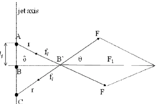
Reneker et al. [42] described the first order instability using the Earnshaw theorem (Figure 2.3) where three points A, B and C of like charges were considered along the jet axis. Interaction of these three like charges results in a perturbation that moves the point B off the axis (perpendicular to the axis) by a distance δ to B’. Reneker et al. showed that this small perturbation grows exponentially. When this perturbation occurs in a liquid jet, forces such as surface tension and viscoelatic forces attempt to counteract the Coulombic force. However, the Coulombic force dominates,overcoming the viscoelastic forces and surface tension, and thus allows the perturbation to grow as a first order instability.

Figure 2.4. Reneker and Fong [43] presented a prototypical path that the jet follows during its multiple instabilities and showed that the instability follows a cycle of three steps: (1) a smooth segment that is linear or curvilinear suddenly dislocates (bends) from its path due to small perturbation; (2) the segment of the jet within the bend region extends and the jet follows a helical path with increasing diameters; and, (3) as the perimeter of the loops increase, the cross-sectional diameter of the jet grows smaller; and hence, the conditions for step (1) are re-established on a smaller scale, thus the next cycle of bending instabilities begins. Consequently, as a result of multiple instabilities, the jet elongates and the diameter of jet reduces considerably; while doing so, the jet solidifies and ultimately deposits on the collector as a dried nanofiber.

2.5 Electrospinning variables

There are a number of research publications [1,28,44-59] that have studied the effect of variables affecting electrospun fibers and/or mat quality. Figure 2.5 shows a general classification of these variables as: (1) material variables; (2) process variables; and (3) equipment variables. Each variable affects the electrospinning process in one or more ways, and therefore can affect the final fiber quality. In this section, the variables that have significant effect on fiber quality are discussed.

Figure 2.3 Illustration of Earnshaw instability, leading to bending of an electrified jet [42].

Figure 2.4 Representation of multiple instabilities from a single jet

2.5.1 Material variables

2.5.1.1 Polymer concentration and molecular weight

Higher polymer concentration in solution increases the molecular entanglements which raises the bending stiffness of the jet. This stiffness prevents the jet from whipping until thinner diameter jets are established and therefore, lengthens the linear region for the jet. Thus, for a fixed working distance, the whipping region is reduced in size, resulting in a larger fiber diameter (and a smaller area of deposition on collector plate). Conversely, the fiber diameter will decrease with lowering of the polymer concentration, however below some minimum concentration level, the jetting process is not stable and a bead-like morphology is observed [44]. This beading occurs because at lower polymer concentration, there are not enough entanglements between polymer chains to create continuous, uniform fibers. The effect of molecular weight is similar to the concentration, where polymer solutions of higher molecular weight have more entanglements, thus resulting in larger diameter fibers [30, 45, 46, and 60].

2.5.1.2 Solution conductivity

increased solution conductivity a lower applied voltage would be sufficient to initiate a jet. Solution conductivity can be altered by the choice of solvent and/or addition of ions or other charged particles [45, 46].

2.5.1.3 Surface tension

Higher surface tension solutions tend to form beaded fibers. The surface tension of the polymer solution drives the jet to break into multiple droplets, while the viscoelastic forces of the polymer solution acts to maintain a continuous or stable jet. When the surface tension is higher than the viscous forces, beaded fibers are produced, similar to the process previously discussed for low concentration solution where beaded fibers were observed when there are not enough polymer chain entanglements (viscous forces). In general, polymer solutions of low surface tension are preferred for electrospinning [1, 38].

2.5.1.4 Other material variables

In addition to the variables listed above, solvent vapor pressure, density of the solution, elasticity [54] are other variables can have a minor effects on the resulting fiber properties [1].

2.5.2 Process variables

2.5.2.1 Applied voltage - Magnitude

Researchers [47, 59] have studied the effect of applied voltage (magnitude) on fiber diameter and observed both increasing and decreasing trends. Increasing the applied voltage draws more fluid from the tip of the needle, thus creating a longer linear region (due to the excess volume of fluid) which results in larger fiber diameters. However, the increased electrical force also increases the whipping instability which raises the frequency of whipping, and thus, counteracts the effect on fiber diameter [28]. In addition, at higher applied voltages multiple jets have been observed, resulting in a larger distribution of fiber diameter. It has also been shown that beaded fibers can be created at increased voltage. At low voltages, less fluid is drawn from the tip of the needle resulting in a shorter linear region and consequently (for a fixed working distance), a longer whipping region [1]. However, the reduced electrical force also decreases the frequency of whipping and counteracts the drawing (elongation) that was expected from the longer whipping region, and hence, (ironically) there is no overall effect on fiber diameter.

2.5.2.2 Applied voltage – Signal and Polarity

Usually a DC high voltage with positive polarity is used in electrospinning. Researchers [55, 56] have observed that the electrospinning process with negative polarity is less efficient and also resulted in beaded and uneven fibers.

reduced whipping instability [49, 51] which could be usefully applied in obtaining multiple jets and avoiding inter-jet interactions.

2.5.2.3 Volume feed rate

Volume feed rate is an important variable that has a significant effect on fiber diameter. Fiber diameter increases significantly with feed rate. However beyond a certain limit, solvent does not evaporate completely resulting in fused fibers or fibrous mat with residual solvent (and hence “wet” polymer) on the collector. At very high feed rates, polymer droplets would drop from the needle, thereby affecting the stable electrospinning process. At a slow feed rate, there is not enough solution for the electrospinning process, eventually resulting in the production of beaded fibers or beads [45, 47].

2.5.2.4 Working distance

2.5.2.5 Other process variables

Other process variables such as electric current, ambient conditions (RH (relative humidity), temperature, vacuum) also affect the fiber morphology. Temperature affects the evaporation rate of the solvent and viscosity of the solution thereby affecting final fiber diameter [57]. Effect of RH depends on the polymer that would increase or decrease the fiber diameter. Investigations at vacuum conditions resulted in little effect on mechanical properties of the fibrous mat [51, 52].

2.5.3 Equipment variables

Most of the equipment variables affect the pattern in which the fibrous materials are collected (aligned, unaligned, tube-like or mat-like forms, etc.). There are a few equipment variables

that affect the fiber diameter; the needle (or nozzle) diameter is one of them. A larger diameter needle supplies a bigger droplet at the needle tip, resulting in larger jet radius and eventually larger fiber diameter [58]. Also, in such cases, multiple jets would be emanating from the needle tip, resulting in irregular fibers. Other equipment variables were already discussed section 2.3.

Ramakrishna et al. [45] studied the effect of various parameters (variables discussed above) and obtained a processing map in which the effects of important process variables are shown in Figure 2.6 [45]. This diagram gives us a general understanding of the major process variables and their effect on fiber diameter.

2.6 Scale up approaches

[62]). Thus, a trade-off must be made between flow rate and field strength. Many researchers have attempted scale-up of the electrospinning process in more sophisticated ways, such as increasing the number of spinning sites. The previously reported approaches can be generally classified based on the feed method at the spinning site: either a confined or unconfined fluid-volume feed as shown in Figure 2.7.

2.6.1 Confined fluid flow

In confined feed systems, the polymer solution is injected at a constant rate (except for a few approaches which are gravity-assisted [64]) into an enclosed capillary (such as a needle or nozzle). High voltage is applied to the enclosure (or nozzle) or directly to the polymer solution using electrodes. Most scale up approaches based on confined feed systems utilize one or more [38, 63, 65-72] nozzles and each nozzle can produce one or more fluid jets, with additional jets formed by use of a grooved tip [12], a curved collector [65], or jet splitting [66]. Electroblown spinning [11] is another confined feed system similar to TNE electrospinning but using a controlled airflow near the lower end of the nozzle to aid in solvent evaporation and thus, allowing spinning at a higher flow rate than usual and an increased production rate.

head with peripherally disposed extrusion tubes [75], a multi-channel microfluidic device [76], and electrospinning using charge injection [77]. In charge injection, when a net charge is injected to the fluid streams, it develops a self-electric field within the stream and stream surrounding it, thus causing breaking into multiple jets. The majority of scale-up approaches reported thus far utilize multiple nozzles with confined feed; hence, essentially, a linear scale-up of needle electrospinning. One of the major advantages of confined feed is the controlled flow rate, which is important for maintaining a continuous stable electrospinning process and controlling the nanofiber diameter (as higher flow rates are generally associated with thicker fibers). However, confined feed systems are innately prone to clogging, and require an engineered structure for each jet (or several jets), thus significantly increasing the complexity of the system [13].

2.6.2 Unconfined fluid flow

used to create bubbles in the polymer solution at which locations jets are formed. Finally, in centrifugal electrospinning, polymer droplets are fed onto a rotating disc and move radially to the rim of the rotating disc, where jetting occurs.

Challenges in unconfined feed systems are control of solution feeding, larger fiber diameter, and wider fiber diameter distribution. Because of the large number of potential jets, inter-jet interactions [48, 68] are a potential challenge for researchers exploring electrospinning scale-up.

2.7 Self-Assembled Monolayer (SAM)

This section introduces a technique -- growth of self-assembled monolayers -- utilized to modify the surface property of the source plate(s) which are used in this work. Self-assembled monolayers are single-molecule-thick collections formed by chemi- or physio-absorption onto a solid substrate [83-86]. In this work, silane precursor molecules are utilized which react with the hydroxyl groups on oxide surfaces and form chemical bonds to the surface (Figure 2.8). SAMs have widespread applications particularly to alter surface wetting properties, which is their main purpose in this work [87]. In this section, we discuss SAM formation technique and an application of SAMs related to the modification of surface wetting properties.

silicon oxide is covered with a hydrophobic collection of alkyl chains. Hydrophobicity of a substrate can be measured by measuring the water contact angle. Figure 2.9 shows typical water contact angles of a substrate before, and after, SAM growth.

Figure 2.9 Representation of water contact angle (θ) of a substrate (a) before SAM and (b) after SAM

(a) (b)

Figure 2.8 Formation of SAM on a silica surface using decyltrichlorosilane

The water contact angle is the internal angle that a droplet makes when placed on a solid surface. Hydrophilic surfaces have small angles (<15º) whereas hydrophobic surfaces have larger values (up to ~120º).

In this work, SAMs are grown from the vapor phase, which provides a disordered surface film where the molecules are uniformly distributed [88]. This technique has been used in this investigation in order to modify the surface wetting properties of the substrate (aluminum with an oxide layer) to assist in electrospinning.

2.8 Electric field simulations

Characterization of the electric field magnitudes and spatial pattern is essential in understanding the electrospinning process. Differences in the geometric configuration of the electrospinning set up affect the electric field distribution. This section outlines a software Maxwell SV 2D that is used for analyzing electric field distribution of different geometries.

Maxwell SV 2D uses finite element analysis (FEA) to solve the problem through the following steps.

i) Automatically creates the required finite element mesh

ii) Iteratively calculates the desired electrostatic field solution until the solution converges.

iii) Provides the ability to analyze, manipulate, and display field solutions.

Chapter 3 Research objectives

Electrospun nanofibers have widespread applications in tissue scaffolds, filtration, protective clothing, and optical electronics. However, the fabrication rate of the traditional needle electrospinning (TNE) process is very limited (on the order of 0.01 - 0.1 g/hr [13]). The scale-up approaches reported tend to be complex and/or can negatively alter the desired fiber morphology and quality. Thus, it is important to identify an approach to fabricate nanofibers with less complexity (still possessing the desired morphologies) and a high potential to scale-up for commercial viability. Towards this goal, obtaining fibers at truly the nanoscale (i.e. < 100 nm) with a narrow diameter distribution is equally important. This work focuses on an approach that shows promise for fabrication of electrospun fibers at the nanoscale from unconfined fluids, and the potential to significantly improve the fabrication rate. The research objectives are outlined below.

1. Investigate the prospect of electrospinning from a flat plate with unconfined fluids and further elucidate the fundamental physical process. This includes:

b. Studying the electric field distributions of prospective geometries and identifying the fundamental requirements to initiate a jet from a proposed geometry.

c. Optimizing the parameters in the proposed geometry to fabricate electrospun nanofibers with morphological properties equal to or better than those in TNE and improved throughput.

d. Establishing processing parameter-fiber property relationships in the proposed geometry.

2. Analyze and compare the physical phenomena of the electrospinning process and the fiber/mat properties of the proposed geometry with respect to the TNE. This includes:

a. Characterizing the jet profiles by imaging the electrospinning process in both the proposed and TNE geometries.

b. Characterizing the morphology of nanofibers using scanning electron microscopy in both the proposed and TNE geometries.

c. Evaluating the spinnability and porosity of nanofiber mats in both the proposed and TNE geometries.

3. Determining the scale-up possibilities of the proposed plate geometry. This includes: a. Evaluating the extent of scale-up possibilities with the proposed plate

geometry.

Chapter 4

Experimental

4.1 Materials

Polyethylene oxide (PEO), with an average weight molecular weight of 400,000 g/mol (400k) (Scientific Polymer Products) was used without further purification. Solutions of 6 weight-percent (wt %) in de-ionized water, stirred for 24 hours at room temperature to aid dissolution, were used for all experiments. Rhodamine 590 chloride (R6G) (Exciton) was used (0.001 wt %) to enhance imaging contrast when viewing the electrospinning process (especially Taylor cone). Viscosity measurements were done using Stresstech instruments RHEOLOGICA Instruments AB at 25º C and zero-shear viscosity was found to be 9250 cP. Polycaprolactone (PCL), with a number average molecular weight of 70,000 – 90,000 (by GPC) (Scientific Polymer Products) was used without further purification. Solutions of 12 weight-percent (wt %) in dimethyformamide (DMF) and dichloromethane (DCM) (solvent ratio 1:1), stirred for three hours at room temperature were used at particular instances which are further discussed in results section.

Figure 4.1 Contact angles measurements for an aluminum plate whose wettability has been chemically modified by treatment with decyltrichlorosilane (C10) for (a)

water (105 ± 3º) and (b) 6 wt % PEO+water spinning solution (87 ± 3º).

(10 minutes with oxygen) to enhance the number of available hydroxyl groups for the film growth reaction and ensure suitable surface cleanliness. These plates are further referred as A type plates. The plates were preheated in an oven for 30 minutes at 90° C then exposed to C10 vapor for 1 hour. During this process, the hydrophilic hydroxyl surface groups react with, and are covered by, the alkyltrichlorosilanes, which ultimately form a disordered monolayer with a hydrophobic methyl and methylene-terminated surface [85]. Plates were rinsed with methanol for 10 seconds and sonicated in toluene for 10 minutes to remove any material not permanently attached to the surface. This process provides a disordered but hydrophobic monolayer-like coating of the metal plate surface. Water contact angle (droplet size 2 μl, average of five readings) on aluminum plate before film growth was ~ 0º (i.e., the water wetted the surface), and after treatment was 105 ± 3º (Figure 4.1a). For the PEO:water

identical plates (12" x 8" x ¼") made of aluminum (McMaster Carr) were used and one of them was treated with C10 in order to obtain a hydrophobic surface. These plates are referred as B type plates.

4. 2 Apparatus

A commercial power supply (Glassman High Voltage Model No. FC60R2) provided positive polarity, high voltage to the source plate (or needle), while the collector plate was held at ground potential. Aluminum foil covered the collector plate in order to gather the electrospun mat samples for further measurements.

For quantitative analysis of the linear and whipping regions of the electrospinning process, a camcorder (Panasonic SDR – H60) (with a 6 mm x 18 mm T monocular (Zeiss) to capture

Taylor cone) recorded images while the polymer jets were illuminated with industrial video lighting equipment (Olympus).

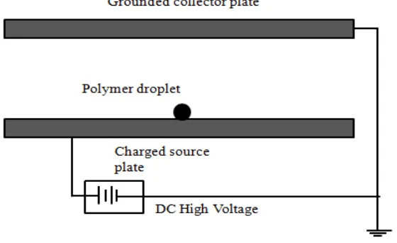
Figure 4.2 shows an initial set up where two identical plates (B type) were placed horizontally separated by certain distance. The source plate treated with C10 was placed at the bottom and connected to power supply while the collector was placed at top and grounded. Two other configurations (in addition to TNE) (which are the principle investigation apparatus) were utilized for electrospinning as shown in Figure 4.3a and 4.3b.

The edge-plate configuration consisted of an aluminum source plate (A type) held at 40º (

to horizontal with a vertical collector plate, as mentioned in previous section and as indicated in Figure 4.3a. Additionally, multiple thin plates (A type) were stacked to form a waterfall spinning configuration (Figure 4.3b) with collector. Each plate was attached to the high voltage power supply. In either configuration, an electrically insulated reservoir fitted with

Pipette

Figure 4.3 (a) Illustration of single edge-plate electrospinning, θ and direction of gravity (Fg),

one or more plastic pipettes supplied polymer solution to the charged plate. For the solution viscosity used here (9250 cP), the solution traveled in a straight line from the pipette down the plate with little branching. All plates were treated with the C10 monolayer as described above. The working distance refers to the distance between the edge of the source plate (bottommost plate in case of waterfall configuration) to the grounded collector plate surface.

4.3 Fiber characterization

Nanofiber morphology was studied with a Phenom SEM (FEI) operating at 5.0 kV. The samples were coated on a S67620 mini sputter coater (Quoron technologies) with Au-Pd at a thickness of 100 Å to reduce charging and produce a conductive surface. The SEM images were analyzed using ImageJ Analyzer software to determine diameter and porosity characteristics; 25 individual measurements made on each sample determined the mean nanofiber diameter and standard deviation.

Porosity is measured using ImageJ Analyzer software by converting SEM images into grey scale where the fibrous area is differentiated from voids. Porosity values are determined as a percent of void area to the total area of the mat. In this analysis, a single layer of the fibrous mat is considered for all samples.

Spinnability is defined as the measure of percent of dry fibrous area to the total area of the fibrous mat. Undried areas are visible and appear like patchy lines on the images of fibrous mat. These portions are marked in different color using MS-paint software and then converted into grey scale using ImageJ analyzer in order to find the percent of the dried fibrous area to the total area of the mat.

4. 4 Electric field simulations

Chapter 5

Results and discussion

5. 1 Electric field simulations

Electric field strength and homogeneity in various electrospinning configurations (using Maxwell SV 2D software as described above) is discussed. Qualitatively, the TNE geometry results in a very inhomogeneous field with the strongest field and field gradient at the needle. Conversely, pure parallel plate geometry (identical plates that are placed horizontally one above the other separated by a certain distance, Figure 4.2) results in a homogeneous field (i.e., no field gradient) at the center of the plates and a lower maximum field compared with TNE. However, within the parallel plate geometry, the sharp edges of the plate can still result in a strong electric field and field gradient at those locations. One could then imagine easily forming many spinning sites along the entire edge; a more facile approach to parallel spinning sites than employing an array of needles. It is observed that since the strongest electric field and the strongest gradient tend to occur at the same location, one goal of this work is to decouple the two effects. As discussed later, the electric field gradient at the location of jet formation appears to be the most important parameter to ensure effective fiber formation. It is important to note that while the electric field can be increased by simply increasing the voltage, the electric field gradient is geometry-specific.

Figure 5.1 Electric field distributions for TNE geometry with 15 cm working distance and 15 kV

For an applied voltage of 15 kV and 15 cm working distance, in the TNE geometry (Figure 5.1), the magnitude of the simulated electric field (E) near the needle tip is 4.2 ± 0.2 x 105 V/m and gradually decreases to 7.5 ± 2.5 x 104 V/m at the collector. Applying the same voltage and working distance in the parallel plate geometry (Figure 5.2), at the center of the source plate E = 1.0 ± 0.2 x 105 V/m and does not vary significantly from that point to the collector (resulting in no electric field gradient). Thus, in comparison, the TNE configuration has a higher field magnitude and a larger field gradient. However, the electric field at the source plate edge (1.3 ± 0.1 x 105 V/m) (in the parallel-plate set up) is higher than between the plate centers and results in a non-zero electric field gradient. These simulated electric field distributions correspond with other reports of the TNE geometry and of unconfined feed electrospinning using cylindrical and disk spinning sources [64, 89]. In

particular, the effect of higher field strength at the plate edges could be compared to the cylindrical nozzle edges which displayed a higher magnitude electric field than that at the center of the cylinder.

The higher electric field exhibited at the plate edge can thus be utilized more efficiently in the edge-plate geometry (Figure 5.3). In the edge-plate geometry, for the same voltage and working distance, the maximum field is quite similar to that in the TNE configuration in magnitude and gradient, that is 4.3 ± 0.3 x 105 V/m at the edge and gradually decreasing to 7.5 ± 2.3 x 104 V/m at the collector. This indicates that the edge-plate geometry could be a direct substitute for TNE but with many more potential spinning sites. However, even though the electric field parameters are similar, in the edge-plate scenario, an unconfined flow of polymer solution over the surface of the plate might alter the stability, effective flow rate, and size and shape of the linear and whipping regions during spinning and thus the resultant nanofiber quality, such as the average fiber diameter and diameter distribution. The results discussed below that indicate these factors can be overcome and that nanofibers spun from the same solution in TNE and edge-plate configurations have very similar diameter distribution and average size. However, higher mass throughput is obtained when utilizing the edge-plate configuration.

5.2 Jet formation

10 cm working distance (2.5 x 105 V/m). Even when the electric field at the plate center was tuned (by increasing the applied voltage) so that it was the same magnitude as that for successful spinning from the edges, no jetting was observed from the plate center. To summarize, in regions where the electric field is highly homogeneous no jet formation was observed, for a wide range of applied electric fields and two different viscosity solutions. On the other hand, jet formation was seen for both solution types near the plate edges. Therefore, the electric field inhomogeneity (i.e., a field gradient) in these regions favors jet formation, as also discussed by Yang et al. [28].

Figure 5.4 PEO-polymer solution droplet (doped with R6G) falling from the plate, and the subsequent jet initiation process. Sequential video images taken under room light illumination. Arrows in the images (d, e and f) shows the jet direction.

on and off the plate (Figure 5.4c.) and the pendent droplet elongates. The simultaneous elongation of the fluid (Figure 5.4d.) and presence of the strong electric field and electric field gradient at the plate edge couple to create jet initiation (Figure 5.4e.). The jet from the Taylor cone forms a linear region followed by a whipping region in analogy to the TNE process.

however, in those experiments, no jet formation was observed.) The successful jetting process here is a result of the combined effect of the thinning of the polymer solution due to gravity and the field gradient at the plate edge. In a recent work [89] on needleless electrospinning (using a rotating cylinder (that provides a lesser gradient at the cylinder edges)) with polyvinyl alcohol (9.0 wt % in distilled water) solutions of 1620 cP viscosity, for stable electrospinning, an electric field of 5.8 ± 0.4 x 105 V/m (computed using the reported spinning parameters for Maxwell SV 2D simulations. In contrast, in the PEO experiments reported here with a significantly higher viscosity (9250 cP) solution, the minimum electric field at the jet location is slightly less and comparable to TNE which is 4.6 ± 0.2 x 105 V/m for 35 cm working distance. Thus edge-plate geometry provides a sharp electric field gradient at the edge that assists in the initiation of jets at electric potentials similar to TNE process. In addition, thinning of the polymer solution by gravity also assists in jet initiation.

observed when θ = 40º (as discussed above), above which there was an excessive supply that caused frequent drip off and below which the jet was depleted of polymer solution. Both solution scarcity and excess resulted in extinction and re-creation of the jet, and thus an intermittent rather than continuous electrospinning process.

5.3 Jet profiles

Jet profiles for TNE and edge-plate electrospinning were compared; Table 5.1 summarizes the length of the linear region, cone angle (full cone angle) of the whipping region and the diameter of the resultant mat on the collector. Also for each configuration, the electric field at the tip of the source (needle or edge) and near the collector is specified to develop an understanding of electric field distribution while studying the jet profiles. Discussion in this section is focused on the linear region, the whipping region and the factors affecting each.

Table 5.1 Electric field strength and jet profiles measurements of TNE and edge-plate electrospinning process.

As shown in Table 5.1, for a normal working configuration, needle electrospinning has a small linear region which represents ~22% of the total working distance. In TNE, the linear region length, L, is given by Equation 4 [40,43] (as discussed in section 2.4.2) where K is the solution conductivity, Q is the feed rate, ρ is solution density, χ is the aspect ratio of jet, Eα is

local electric field strength, I is electric current and έ is the dielectric constant. In TNE, the size of the linear region with different feed rates (5, 7.5, 10 and 12.5 µl/min) keeping the electric field and working distance constant were studied. These results also show that increasing feed rate increases the linear region. Subsequently, this reduces the length of the

whipping region and so the jet spends less time in whipping, resulting in larger nanofiber diameters. In Figure 5.5a, the effect of feed rate on length of the linear region (in % of the total working distance, left ordinate) and fiber diameter (right ordinate) and are presented. In TNE, it is observed that fiber diameter increased as the feed rate was increased up to 12.5 µl/min. (At feed rates greater than this, solvent evaporation is not complete and residual solvent is deposited on the collector.) In edge-plate geometry, the linear region is longer, approximately 28% of the total working distance (Table 1). The increase in the linear region is due to the higher flow; a similar trend is seen in TNE under similar conditions (voltage (28 kV) and working distance (35 cm) with a larger needle diameter-to accommodate greater fluid volume) as a function of feed rate, as shown in Figure 5.5b. There are two important observations from this comparison. First, there is no statistical difference (within the

L5 ₌ K

4_Q7_ρ3_(lnχ2₎

8π2_E

αI5(έ)2

Figure 5.5 (a) Average fiber diameter and jet linear region length vs. feed rate in (a) TNE process with 15 cm working distance and 11 kV (b) TNE and Edge plate electrospinning process with 35 cm working distance and 28 kV.

standard deviation) for the length of the linear region and the average fiber diameter between the two methods; second, for TNE, there is a discontinuous change (drop) in the fiber diameter as the spinning parameters are changed to accommodate the higher feed rates.

Figure5. 6: (a) Schematic representation of jet in plate electrospinning (b) Image of jet profile at 35 cm working distance

Figure 5.7: Amplitude A of whipping instability as measured from the radius of the instability envelope vs. axial distance (z) from the onset of whipping instability fit to an exponential function. Shin’s whipping trend is shown with a dotted line in conjunction with the primary and secondary cones observed in TNE and edge-plate electrospinning for this work.

It is germane to note that the secondary cone is only seen at working distances of 35 cm or greater (for both TNE and edge-plate). Shin et al. [90] quantified the cone envelope as a function of distance from the onset of the cone and found it fit an exponential function. Figure 5.7 shows the Shin data (for PEO and water (where only a primary cone angle was observed)) along with our TNE and edge-plate configurations. Here, the cone envelope for the secondary cone is also plotted, which is also exponential, but fits with different coefficients than the primary cone (i.e. it is discontinuous). Therefore, it is clear that the secondary cone is a unique feature for longer working distance electrospinning (for both TNE and edge-plate). This secondary cone might be associated with subsequent cycles of bending instabilities (as discussed by Reneker et al.) [42], and therefore, is more easily observed at longer working distances. This hypothesis supports the above observation (Figure 5b) that at working distances above 35 cm (where the secondary cone is visible and hence more whipping takes place) the fiber diameter drops below that for working distances less than 35 cm.

5.4 Processing parameters-fiber properties relationships

5.4.1 Fiber diameter and diameter distribution

5.4.1.1 Effect of fluid flow

104 V/m) and a feed rate of 30 µl/min, edge-plate electrospinning resulted 275 ± 32 nm. The mean diameter of the edge-plate electrospun fibers is approximately 10% bigger and the standard deviation is larger than that for the optimized TNE process. The increase in the fiber diameter is likely due to the higher feed rate. As discussed in section 5.3, higher feed rates increase the linear region which decreases the whipping region and results in a larger fiber diameter. When edge-plate is compared to TNE under similar conditions (35 cm working distance, 28 kV and 30 µl/min) the resulting TNE nanofibers have an average diameter of 292 ± 28 nm, which is slightly larger but overlaps with that for the edge-plate electrospun fibers. Thus, we conclude that the primary reason for the increase in the average fiber diameter typically reported for unconfined systems is due to the increased feed rate.

Figure 5.8: Comparison of electrospun nanofibers from (a) TNE geometry at 15 cm working distance and 11 kV (b) edge-plate geometry at 35 cm working distance and 28 kV.

In previous work [78, 89, and 91] where PEO and other polymer nanofibers were electrospun using different unconfined geometries, fiber diameters were found in the range between 200 - 800 nm with very large standard deviations. It was reported [89] that larger fiber distribution using a cylindrical nozzle was due to the difference in the electric field magnitude at the edges and center of the cylinder which produced finer and coarser fibers respectively. Another reason for larger fiber diameter and distribution could be the unconfined fluid flow rate (and resulting volume accumulation). In most of the unconfined geometries, the fluid flow at the spinning site is seldom controlled. In edge-plate geometry, these issues were overcome. The electric field magnitude and gradient is constant at the spinning sites (the plate edge); and the fluid flow to the spinning site can be controlled by fluid viscosity, pipette diameter, and plate angle. Thus it is facile to tailor the edge-plate parameters to achieve fiber diameters and diameter that are similar to TNE process.

5.4.1.2 Effect of applied voltage and working distance

diameter of electrospun materials was not significantly affected by applied electric field, consistent with the results from edge-plate spinning.

5.4.2 Spinnability and Porosity

In TNE, at very high feed rates (more than 12.5 µl/min at 15 cm working distance and 11 kV, as discussed in section 4.3) solvent evaporation is not complete and the residual solvent deposits on the collector.

In both TNE (up to a 12.5 µl/min feed rate with 15 cm working distance and 11kV) and single edge-plate electrospinning (up to a 45 µl/min feed rate with working distance 35 cm and 28 kV), spinnability values were 100%. However, at a 55 µl/min feed rate, solvent evaporation during jetting was not complete; in addition, the higher throughput caused intermittent spinning that resulted in streaming (discussed in 4.5.2) and spinnability was found to be 98.5%. Also shorter working distances (25 cm) in edge-plate geometry (at different feed rates) did not allow for sufficient solvent evaporation, resulting in an average spinnability of 97.0%.

the longer the working distance, the higher the porosity. This was confirmed with the TNE fibers electrospun at longer working distance (35 cm) at same average electric field which was 70.0 % ± 3.0%. Also it is evident from the previous discussion that increased working distance increases the whipping cone angle and this eventually gives a well spread collection on the grounded collector. Hence, the overall porosity of the nanofibrous mats increases as the working distance increases.

5.4.3 Effect of multiple feed streams on morphology and production rate

Up until this point, spinning has occurred from a single source (i.e,. a single pipette creating one fluid stream). Here, the effect of several pipettes, and therefore multiple fluid streams on the fiber morphology and production rate are discussed. Table 5.2 summarizes the set of

experiments that were done with 35 cm working distance, 28 kV and 30 µl/min (using a pipette size of 1.5 mm). Uniform electric field magnitude and gradient is ensured at all

Number of pipettes distance between Center to center pipettes (cm)

Average fiber diameter (nm)

Fabrication rate (gm/hr)

1 - 275 ± 32 0.13

2 4.8 278 ± 28 0.24

3 2.4 290 ± 41 0.27

5 1.2 311 ± 54 0.19

spinning sites by having the fluid stream away from the corners of the plate (corners of the plate have higher electric field magnitude and gradient).

spinning sites using multiple pipettes on a single plate would be more successful at optimal center to center distance.

5.5 Spinning from multiple plates

Multiple jets could be also initiated by providing multiple spinning sites by utilizing more than one source plate. Several configurations were studied with different possible combinations of plates separated by 10 mm (up to four) as shown in Figure 4.3b and of multiple feed streams (up to three pipettes, spacing as mentioned in 5.4.3). In each configuration, the plates are treated with C10 and held at identical voltages with a feed rate of 45 µl/min (using a 2.0 mm pipette). In this configuration, the use of multiple pipettes provided multiple spinning sites on the first or topmost plate and then the fluid flowed down to subsequent plates, thus creating multiple spinning sites at each of four plates (cascade arrangement). However in all these configurations, it is noticed that the jets were more stable and continuous from the leading edges of the plates (in this case the bottom most plate) than other edges. In this section, this effect is discussed using electric field simulation. The effects of multiple plates and feed streams on fiber morphology and production rate are also discussed.

5.5.1 Electric field Simulation

steepest gradient compared to the other plate edges (2.8 ± 0.2 x 105 V/m). The field strength at the collector was 8.3 ± 1.7 x 104 V/m (for an applied voltage of 32 kV). This complex electric field magnitude and gradient at the spinning sites, therefore, affect the jet initiation, jet profiles, and therefore, the average fiber diameter and diameter distribution. In the following sections these results and discussions of the multi-plate experiments are summarized. This result highlights the crucial importance of the electric field gradient at the edge of plate.

5.5.2 Experimental observations

Jets from the spinning sites at the bottommost plate edges displayed jet profiles similar to that of the single edge (due to similar electric field magnitude and gradient as single edge-plate) but jets from other spinning sites displayed shorter linear regions (~20%) and a smaller whipping cone angle (~30º full cone angle) with no secondary cone (due to less volume of liquid taken by the jet). All these variations contribute to producing larger average fiber diameters and a wider diameter distribution (290 ± 54 nm) for a working distance of 35 cm and 28 kV. Spinnability and porosity found to be 96.0% (due to intermittent spinning) and 69.0 ± 3.0 %, respectively.

5.5.3 Intermittent spinning in TNE

To better understand the intermittent electrospinning, a similar cycle (15 seconds of spinning with a two second interval) with TNE at 28 kV and a 35 cm working distance was studied. In such cases, nanofiber mat with some wet regions (caused by streaming) were obtained. The fiber diameter was found to be 325 ± 40 nm, which is relatively higher than that for the continuous TNE process (keeping all parameters the same) (292 ± 28 nm). Hence the increase in the fiber diameter (and diameter distribution) for the multiple-plate configuration can be attributed to the intermittent spinning and resultant streaming phenomenon.

5.5.4 Fabrication rate

difference in the electric field strength and gradient as discussed in 5.5.1. Fabrication rate for this configuration was found to be 0.153 gm/hr, lower than a two fluid streams from a single edge-plate. These results help to encourage investigating techniques with more focus on providing multiple spinning sites on a single edge-plate, or finding an optimum distance between plates where the electric field magnitude and gradient will be identical at all plates edges.

5. 6 Spinning from edge-cylinder

In this section, a new geometry, an extension of aforementioned concepts, edge-cylinder is introduced. Results of preliminary experiments using edge-cylinder geometry are summarized.

5.6.1 Experimental

5.6.2 Electric field simulation

Maxwell SV 2D was used to model the electric field distribution of the edge-cylinder geometry with a 15 kV and 15 cm working distance (from the surface of the source to the collector cylinder). Figure 5.10 shows the electric field distributions in edge-cylinder geometry as a planar cross-section. Electric field magnitude at the edge of the bowl was found to be 3.3 ± 0.3 x 105 V/m and 6.8 ± 2.2 x 104 V/m at the collector. Thus the edges of the bowl provide a strong electric field magnitude and gradient similar to TNE and edge-plate.

5.6.3 Preliminary results

In order to initiate the jets, a high voltage in magnitude and gradient (45 kV; i.e.,8.8 ± 0.7 x 105 V/m) was required at the bowl edge.

Figure 5.9 Representation of edge-cylinder electrospinning set up Charged bowl

This is probably due to the absence of gravitational flow of fluid which (when falling) would thin down to a fine shape that assists in launching a jet. In edge-cylinder, upon application of this high voltage, the strong electric field at the edge of the bowl propels multiple jets along its edges (forming a radial pattern), however, at these field values, unfortunately, electrospraying to the collector. When the voltage is decreased to 14 kV (3.3 ± 0.3 x 105 V/m), continuous electrospinning was established. Approximately 30 jets were spinning radially from the edge of the bowl and fibers were deposited on to the cylindrical collector. These jets self-organized along the edges of the bowl, approximately equal distance between them. As well, the jets were propelling at an angle (~30º) from the bowl that more or less correlates with the observed pattern of electric field distribution (the arrow drawn in Figure 5.10b).

(b)

(a)

Figure 5.10 (a) Electric field distributions of edge-cylinder geometry (b) magnified image of the edge.

SEM Images of the edge-cylinder electrospun fibers is shown in Figure 5.11. Nanofibers sizes were measured to be 251 ± 25 nm, very similar to those formed under TNE. Also, as the working distance was short, no secondary whipping regions were observed (also similar to TNE). In addition, spinnability in edge-cylinder was 100% (excluding the initial electrospraying events). For future improvement, a method needs to be established to eliminate these initial electrospraying events, or present a new collector surface once the electrospinning starts.

Chapter 6 Conclusions

In this work, a simple geometry, edge-plate, is presented for fabricating nanofibers from gravity-assisted unconfined fluids. The edge-plate geometry provides a strong electric field magnitude and gradient at the spinning site similar to the needle-plate geometry (TNE), but a large area to accommodate multiple spinning sites and no aperture that can clog. The significance of electric field gradient as an important parameter for jet initiation is demonstrated with parallel plate geometry experiments.

Electrospun nanofibers from unconfined fluids using edge-plate geometry are similar in diameter (275 ± 32 nm) to that from TNE (243 ± 19.2 nm). Jet profiles including the linear and whipping regions showed similar trends in both geometries. At longer working distance, an extended whipping region is observed in both geometries. Properties of nanofibrous mat such as spinnability and porosity were investigated as a function of electric field strength and geometry and the process is stable over a range of experimental conditions.

bottommost edge thereby displaying relatively stable electrospinning only from these edges. Intermittent electrospinning was observed in this configuration, thereby affecting the average fiber diameter, diameter distribution and spinnability of the nanofibrous mats.