Digital Filter Design Using Improved Teaching-Learning-Based Optimization

(1)

University of Windsor University of Windsor

Scholarship at UWindsor

Electronic Theses and Dissertations Theses, Dissertations, and Major Papers

9-12-2019

Digital Filter Design Using Improved Teaching-Learning-Based

Optimization

Miao Zhang

University of Windsor

Follow this and additional works at: https://scholar.uwindsor.ca/etd

Recommended Citation Recommended Citation

Zhang, Miao, "Digital Filter Design Using Improved Teaching-Learning-Based Optimization" (2019). Electronic Theses and Dissertations. 7856.

https://scholar.uwindsor.ca/etd/7856

This online database contains the full-text of PhD dissertations and Masters’ theses of University of Windsor students from 1954 forward. These documents are made available for personal study and research purposes only, in accordance with the Canadian Copyright Act and the Creative Commons license—CC BY-NC-ND (Attribution, Non-Commercial, No Derivative Works). Under this license, works must always be attributed to the copyright holder (original author), cannot be used for any commercial purposes, and may not be altered. Any other use would require the permission of the copyright holder. Students may inquire about withdrawing their dissertation and/or thesis from this database. For additional inquiries, please contact the repository administrator via email

(2)

Digital Filter Design Using Improved Teaching-Learning-Based Optimization

By

Miao Zhang

A Dissertation

Submitted to the Faculty of Graduate Studies

through the Department of Electrical and Computer Engineering in Partial Fulfillment of the Requirements for

the Degree of Doctor of Philosophy at the University of Windsor

Windsor, Ontario, Canada

2019

(3)

Digital filter design using improved teaching-learning-based optimization

by

Miao Zhang

APPROVED BY:

______________________________________________ W. Zhu, External Examiner

Concordia University

______________________________________________ Z. Kobti

School of Computer Science

______________________________________________ C. Chen

Department of Electrical and Computer Engineering

______________________________________________ H. Wu

______________________________________________ H. K. Kwan, Advisor

(4)

iii

DECLARATION OF ORIGINALITY

I hereby certify that I am the sole author of this thesis and that no part of this thesis has been published or submitted for publication.

I certify that, to the best of my knowledge, my thesis does not infringe upon anyone’s copyright nor violate any proprietary rights and that any ideas, techniques, quotations, or any other material from the work of other people included in my thesis, published or otherwise, are fully acknowledged in accordance with the standard referencing practices. Furthermore, to the extent that I have included copyrighted material that surpasses the bounds of fair dealing within the meaning of the Canada Copyright Act, I certify that I have obtained a written permission from the copyright owner(s) to include such material(s) in my thesis and have included copies of such copyright clearances to my appendix.

(5)

iv

ABSTRACT

Digital filters are an important part of digital signal processing systems. Digital filters are divided into finite impulse response (FIR) digital filters and infinite impulse response (IIR) digital filters according to the length of their impulse responses. An FIR digital filter is easier to implement than an IIR digital filter because of its linear phase and stability properties. In terms of the stability of an IIR digital filter, the poles generated in the denominator are subject to stability constraints. In addition, a digital filter can be categorized as one-dimensional or multi-dimensional digital filters according to the dimensions of the signal to be processed. However, for the design of IIR digital filters, traditional design methods have the disadvantages of easy to fall into a local optimum and slow convergence.

(6)

v

obtained by the two improvements have demonstrated their efficiency and effectiveness.

(7)

vi

ACKNOWLEDGEMENTS

I would first like to thank my supervisor, Dr. H. K. Kwan, for suggesting the research topics, the TLBO algorithm, and their design improvements, as well as for editing the write-up of my dissertation.

I would also like to acknowledge Dr. Ziad Kobti, Dr. Chunhong Chen and Dr. Huapeng Wu for their comments on my dissertation. I am grateful to Dr. Weiping Zhu, University of Concordia, for serving as my External Examiner.

I would like to thank my fellow graduate student Jiajun Liang for discussions.

(8)

vii

TABLE OF CONTENTS

DECLARATION OF ORIGINALITY ... iii

ABSTRACT ... iv

ACKNOWLEDGEMENTS ... vi

LIST OF TABLES ... x

LIST OF FIGURES ... xv

LIST OF ABBREVIATIONS/SYMBOLS ...xxiiii

CHAPTER 1 Introduction... 1

1.1 FIR and IIR digital filters ... 1

1.1.1 FIR Filters ... 2

1.1.2 IIR Filters ... 4

1.2 Two dimensional digital filters ... 6

1.3 Optimization algorithms ... 8

1.4 Motivations of the dissertation ... 10

1.5 Organization of the dissertation ... 10

1.6 Main contributions ... 11

CHAPTER 2 Teaching-Learning-Based Optimization and Improved Algorithms 13 2.1 Review of swarm intelligence algorithms ... 13

2.2 Literature review of TLBO algorithm ... 17

2.3 Teaching-learning-based optimization ... 20

2.4 Gradient-based TLBO Algorithm ... 22

CHAPTER 3 Linear phase FIR filter design ... 26

3.1 Problem formulation ... 26

3.1.1 Type 3 Linear Phase FIR Filters ... 26

3.1.2 Type 4 Linear Phase FIR Filters ... 28

3.1.3 Hilbert Transformer ... 29

3.1.4 Objective Functions ... 29

(9)

viii

3.1.4.2 Least square design ...29

3.2 Designs and Results ... 30

3.2.1 Type 3 bandpass HT MM designs ... 30

3.2.2 Type 4 highpass HT MM designs ... 36

3.2.3 Type 3 bandpass HT LS designs ... 42

3.2.4 Type 4 highpass HT LS designs ... 50

3.2.5 Comparison with references [1] ... 58

3.3 Analysis ... 62

3.4 Conclusions ... 62

CHAPTER 4 General FIR Digital Filter Design using Multiobjective TLBO algorithm ... 64

4.1General FIR digital filter design ... 65

4.1.1 General FIR digital filters ... 65

4.1.2 Objective Functions ... 66

4.1.2.1 LS error ...66

4.1.2.2 Minimax error ...67

4.2 MOPSO Algorithm ... 68

4.2.1 Basic Concepts ... 68

4.2.2 MOPSO ... 68

4.3 MOTLBO algorithm based on non-dominated solutions... 71

4.4 Gradient-based MOTLBO Algorithm ... 74

4.5 General FIR digital filter Design examples ... 76

4.5.1 Minimax design using non-dominated MOTLBO ... 77

4.5.2 Least squares design with gradient-based MOTLBO ... 83

4.6 Analysis ... 90

CHAPTER 5 IIR Digital Filter Design Using Multiobjective TLBO Algorithm ... 92

5.1 IIR Filter Design Problem ... 93

5.1.1 IIR digital filters ... 93

5.1.2 Stability constraints ... 93

5.1.3 Objective function ... 93

5.2 Euclidean-Distance-Based MOTLBO ... 96

(10)

ix

5.4 Analysis ... 102

CHAPTER 6 2-Dimensional Linear Phase FIR Digital Filter Design using TLBO Algorithm ... 104

6.1 2-D Linear Phase FIR Filter Design Problem ... 105

6.1.1 Digital filter transfer function ... 105

6.2 Design examples ... 106

6.2.1 Example 1 ... 108

6.2.2 Example 2 ... 113

CHAPTER 7 Two-Dimensional Nonlinear Phase FIR filters Design ... 120

7.1 2-D Nonlinear Phase FIR Filter Design Problem ... 121

7.1.1 2-D FIR digital filter ... 121

7.2 Filter Design and design examples ... 122

CHAPTER 8 Conclusions and Future Study ... 134

8.2 Future works ... 135

REFERENCES/BIBLIOGRAPHY... 137

(11)

x

LIST OF TABLES

Table 3.1 FIR Filter and TLBO (Gradient-based TLBO) Parameters (Key: LP-FIR 3: type 3 Hilbert transformer)………..…31

Table 3.2 Frequency Grid and Desired Amplitude Response……….31

Table 3.3 Hilbert transformer minimax errors (Keys: : Type; BP: Bandpass; HP: Highpass; : Filter order; : Algorithm; 1: firpm.m; 2: TLBO; CPU: Time in sec)………. .31

Table 3.4 Hilbert transformer minimax peak error (Keys: : Type; BP: Bandpass; : filter orders; MM: Minimax; : Algorithm; 1: firpm.m; 2: TLBO; : Peak error frequency; C: Converged iteration number)………….………32

Table 3.5 FIR Filter and TLBO (Gradient-based TLBO) Parameters (Key: LP-FIR 4: type 4 Hilbert transformer)………...37

Table 3.6 Frequency Grid and Desired Amplitude Response………..37

Table 3.7 Hilbert transformer minimax errors (Keys: : Type; HP: Highpass; : Filter order; : Algorithm; 1: firpm.m; 2: TLBO; CPU: Time in sec)………..……… …37

Table 3.8 Hilbert transformer minimax peak error (Keys: : Type; HP: Highpass; : filter orders; MM: Minimax; : Algorithm; 1: firpm.m; 2: TLBO; : Peak error frequency; C: Converged iteration number)………....38

Table 3.9 Hilbert transformer LS Design Results (A: algorithm; 1: firls.m; 2: TLBO algorithm; 3: gradient-based TLBO algorithm; Iter: Iteration; LS: Least square algorithm; C: Converged iteration number; CPU: Time in sec)...43

Table 3.10 Filter Coefficients of T3-N14………...44

(12)

xi

algorithm; C: Converged iteration number; CPU: Time in sec)... 44

Table 3.12 Filter Coefficients of T3-N26………..…..46

Table 3.13 Hilbert transformer LS Design Results (A: algorithm; 1: firls.m; 2: TLBO algorithm; 3: gradient-based TLBO algorithm; Iter: Iteration; LS: Least square algorithm; C: Converged iteration number; CPU: Time in sec)………..…46

Table 3.14 Filter Coefficients of T3-N38………...…………..48

Table 3.15 Hilbert transformer LS Design Results (A: algorithm; 1: firls.m; 2: TLBO algorithm; 3: gradient-based TLBO algorithm; Iter: Iteration; LS: Least square algorithm; C: Converged iteration number; CPU: Time in sec)……….. 48

Table 3.16 Filter Coefficients of T3-N50………..………..50

Table 3.17 Hilbert transformer LS Design Results (A: algorithm; 1: firls.m; 2: TLBO algorithm; 3: gradient-based TLBO algorithm; Iter: Iteration; LS: Least square algorithm; C: Converged iteration number; CPU: Time in sec)………..51

Table 3.18 Filter Coefficients of T4-N13……….…52

Table 3.20 Filter Coefficients of T4-N25………...54

(13)

xii

Table 3.23 Hilbert transformer LS Design Results (A: algorithm; 1: firls.m; 2: TLBO algorithm; 3: gradient-based TLBO algorithm; Iter: Iteration; LS: Least square

algorithm; C: Converged iteration number; CPU: Time in sec)...56

Table 3.24 Filter Coefficients of T4-N49………...…..58

Table 3.25 FIR Filter Parameters (Key: LP-FIR 3: type 3 Hilbert transformer)……….……59

Table 3.26 Passband frequency grid and points for optimization and evaluation……….. .……….59

Table 3.27 Least squares errors of30th-order linear phase FIR Hilbert transformer design (Keys: : Type; BP: Bandpass; : Algorithm; 1: firls.m; 2: TLBO; 3: Gradient-based TLBO; CPU: Time in sec; Iter: Iteration; LS: Least squares algorithm; C: Converged iteration number; CPU: Time in sec)………..…59

Table 3.28 Filter Coefficients of T3-N30……….61

Table 4.1 General FIR filter and MO parameters……….77

Table 4.2 General FIR filter bound limits………...77

Table 4.3 Cutoff frequencies (LP: Lowpass; HP: Highpass; BP: Bandpass; BS: Bandstop; PB: Passband; SB: Stopband; Gd: Group delay)………77

Table 4.4 General FIR filter minimax errors (Alg: 1. MOTLBO; 2: MOPSO; MM_mag: Minimax magnitude error; MM_gd: Minimax group delay error; CPU: Time in sec)……….……78

Table 4.5 General FIR filter minimax peak errors (Alg: 1. MOTLBO; 2: MOPSO; PB: passband; Gd: Group delay)……….….78

(14)

xiii

Table 4.7 General lowpass FIR filter least squares errors (Alg: 1. Gradient-based TLBO; 2: MOTLBO; 3: MOPSO; LS_mag: Least squares magnitude error; LS_gd: Least squares group delay error; CPU: Time in sec)………...84

Table 4.8 General lowpass FIR filter least squares peak errors (Alg: 1: gradient-based MOTLBO; 2: MOTLBO; 3: MOPSO; PB: passband; Gd: Group delay)………..…….84

Table 4.9 Gradient-based MOTLBO LS coefficients of LP………....85

Table 4.10 General FIR highpass filter least squares errors (Alg: 1. Gradient-based TLBO; 2: MOTLBO;3: MOPSO; LS_mag: Least squares magnitude error; LS_gd: Least squares group delay error; CPU: Time in sec)………..….86

Table 4.11 General highpass FIR filter least squares peak errors (Alg: 1: gradient-based MOTLBO; 2: MOTLBO; 3: MOPSO; PB: passband; Gd: Group delay)…...86

Table 4.12 Gradient-based MOTLBO LS coefficients of HP………..87

Table 4.13 General bandpass FIR filter least squares errors (Alg: 1. Gradient-based TLBO; 2: MOTLBO;3: MOPSO; LS_mag: Least squares magnitude error; LS_gd: Least squares group delay error; CPU: Time in sec)………88

Table 4.14 General bandpass FIR filter least squares peak errors (Alg: 1: gradient-based MOTLBO; 2: MOTLBO; 3: MOPSO; PB: passband; Gd: Group delay)………...…88

Table 4.15 General bandpass FIR filter least squares peak errors (Alg: 1: gradient-based MOTLBO; 2: MOTLBO; 3: MOPSO; SB 1: stopband_1; SB 2: stopband_2)……….88

Table 4.16 Gradient-based MOTLBO LS coefficients of BP……….……89

Table 5.1 IIR Digital Filter Specifications………98

(15)

xiv

Table 5.3 Highpass Filter Design Results (PB: passband; SB: stopband; Gd: group

delay)………98

Table 5.4 Bandpass Filter Design Results (PB: passband; SB: stopband; Gd: group delay)………...99

Table 6.1 Cutoff Frequencies of 2-D FIR Lowpass Filters………109

Table 6.2 2-D FIR Lowpass Filter Design Results……….109

Table 6.3 Computational Requirements……….109

Table 6.4 Cutoff Frequencies of 2-D FIR Lowpass Filters………...113

Table 6.5 2-D FIR Lowpass Filter Design Results……….114

Table 6.6 2-D FIR Lowpass Filter Design Results Using TLBO………..114

Table 6.7 Computational Requirements………...114

Table 7.1 Cutoff Frequencies of 2-D Nonlinear Phase FIR Lowpass Filters……..123

Table 7.2 2-D Nonlinear Phase FIR Lowpass Filter Design Results………..123

(16)

xv

LIST OF FIGURES

Fig.1.1 Structures of direct form I IIR digital filters……….5

Fig. 1.2 Structures of direct form II IIR digital filters………...5

Fig. 1.3 Structures of cascade form IIR digital filters………...6

Fig. 2.1 Flowchart of gradient-based TLBO algorithm……….…...23

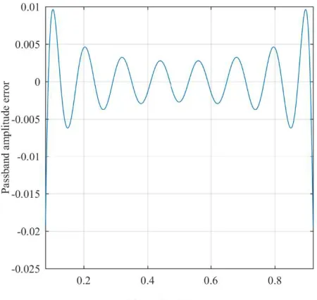
Fig. 3.1 Hilbert transformer minimax design for Type 3 N =14 (a) Amplitude response, (b) Impulse response, (c) Passband amplitude response………...32

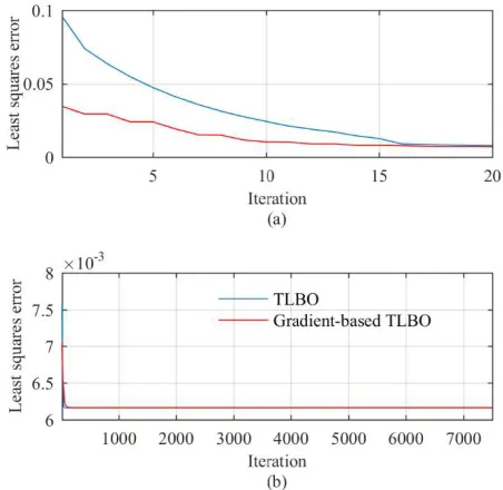
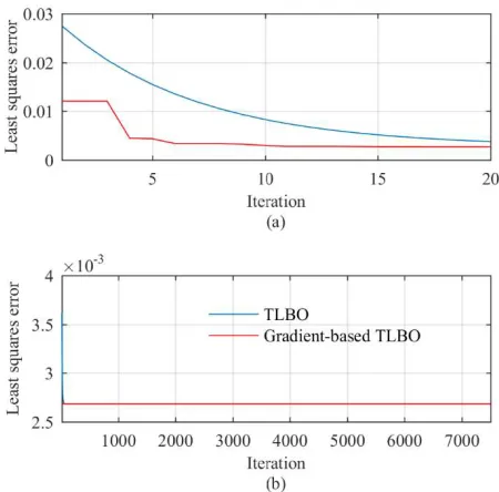
Fig. 3.2 Convergence curve of minimax error for Hilbert transformer design for Type 3 N =14 (a) Interval 1, (b) Interval 2………..…..33

Fig. 3.3 Hilbert transformer minimax design for Type 3 N =26 (a) Amplitude response, (b) Impulse response, (c) Passband amplitude response………...…33

Fig. 3.4 Convergence curve of minimax error for Hilbert transformer design for Type 3 N =26 (a) Interval 1, (b) Interval 2………..….34

Fig. 3.5 Hilbert transformer minimax design for Type 3 N =38 (a) Amplitude response, (b) Impulse response, (c) Passband amplitude response………..34

Fig. 3.6 Convergence curve of minimax error for Hilbert transformer design for Type 3 N =38 (a) Interval 1, (b) Interval 2……….………..35

Fig. 3.7 Hilbert transformer minimax design for Type 3 N =50 (a) Amplitude response, (b) Impulse response, (c) Passband amplitude response…..………35

Fig. 3.8 Convergence curve of minimax error for Hilbert transformer design for Type 3 N =50 (a) Interval 1, (b) Interval 2………36

(17)

xvi

Fig. 3.10. Convergence curve of minimax error for Hilbert transformer design for Type 4 N =13 (a) Interval 1, (b) Interval 2………39

Fig. 3.11. Hilbert transformer minimax design for Type 4 N =25 (a) Amplitude response, (b) Impulse response, (c) Passband amplitude response………..….……39

Fig. 3.12. Convergence curve of minimax error for Hilbert transformer design for Type 4 N =25 (a) Interval 1, (b) Interval 2……….……...40

Fig. 3.13. Hilbert transformer minimax design for Type 4 N =37 (a) Amplitude response, (b) Impulse response, (c) Passband amplitude response………...40

Fig. 3.14. Convergence curve of minimax error for Hilbert transformer design for Type 4 N =37 (a) Interval 1, (b) Interval 2………..……..41

Fig. 3.15. Hilbert transformer minimax design for Type 4 N =49 (a) Amplitude response, (b) Impulse response, (c) Passband amplitude response…………...……41

Fig. 3.16. Convergence curve of minimax error for Hilbert transformer design for Type 4 N =49 (a) Interval 1, (b) Interval 2………....42

Fig. 3.17 Hilbert transformer least squares design for Type 3 N =14 (a) Amplitude response, (b) Impulse response, (c) Passband amplitude response………...………43

Fig. 3.18 Convergence curve of least squares error for Hilbert transformer design for Type 3 N =14 (a) Interval 1, (b) Interval 2………..44

Fig. 3.19 Hilbert transformer least squares design for Type 3 N =26 (a) Amplitude response, (b) Impulse response, (c) Passband amplitude response…………...……45

Fig. 3.20 Convergence curve of least squares error for Hilbert transformer design for Type 3 N =26 (a) Interval 1, (b) Interval 2………...45

(18)

xvii

Fig. 3.22 Convergence curve of least squares error for Hilbert transformer design for Type 3 N =26 (a) Interval 1, (b) Interval 2……….……..47

Fig. 3.23 Hilbert transformer least squares design for Type 3 N =50 (a) Amplitude response, (b) Impulse response, (c) Passband amplitude response………...…49

Fig. 3.24 Convergence curve of least squares error for Hilbert transformer design for Type 3 N =50 (a) Interval 1, (b) Interval 2……….….49

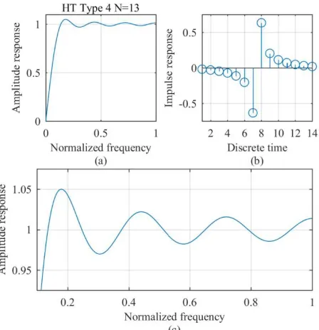
Fig. 3.25 Hilbert transformer least squares design for Type 4 N =13 (a) Amplitude response, (b) Impulse response, (c) Passband amplitude response………..……….51

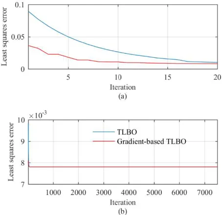
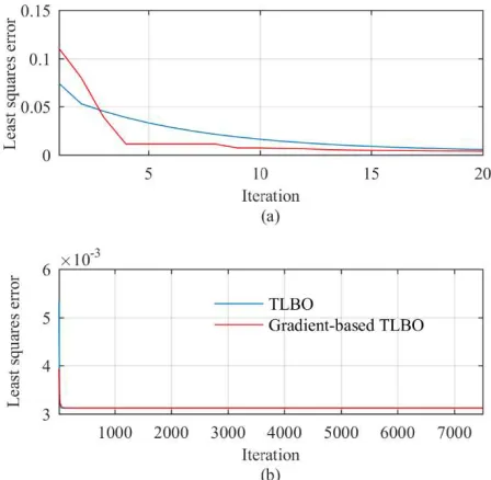
Fig. 3.26 Convergence curve of least squares error for Hilbert transformer design for Type 4 N =13 (a) Interval 1, (b) Interval 2………..….52

Fig. 3.27 Hilbert transformer least squares design for Type 4 N =25 (a) Amplitude response, (b) Impulse response, (c) Passband amplitude response………...53

Fig. 3.28 Convergence curve of least squares error for Hilbert transformer design for Type 4 N =25 (a) Interval 1, (b) Interval 2……….…..53

Fig. 3.29 Hilbert transformer least squares design for Type 4 N =37 (a) Amplitude response, (b) Impulse response, (c) Passband amplitude response………...…55

Fig. 3.30 Convergence curve of least squares error for Hilbert transformer design for Type 4 N =37 (a) Interval 1, (b) Interval 2……….…….55

Fig. 3.31 Hilbert transformer least squares design for Type 4 N =49 (a) Amplitude response, (b) Impulse response, (c) Passband amplitude response………..….57

Fig. 3.32 Convergence curve of least squares error for Hilbert transformer design for Type 4 N =49 (a) Interval 1, (b) Interval 2……….……..57

Fig. 3.33 Hilbert transformer least squares design for Type 3 N =30 (a) Amplitude response, (b) Impulse response, (c) Passband amplitude response……….…..60

(19)

gradient-xviii

based TLBO for Type 3 N =30……….60

Fig. 3.35 Convergence curve of least squares error for Hilbert transformer design for Type 3 N =30 (a) Interval 1, (b) Interval 2……….…61

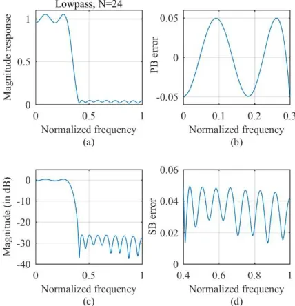
Fig. 4.1 G-FIR LP filter MM design for = 24 and group delay=10 (a) Magnitude response, (b) Passband magnitude error, (c) Magnitude response in dB, (d) Stopband magnitude error………79

Fig. 4.2 G-FIR LP filter MM design for = 24 and group delay=10 (a) Group delay, (b) Passband group delay, (c) Impulse response………....80

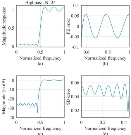
Fig. 4.3 G-FIR HP filter MM design for = 24 and group delay=10 (a) Magnitude response, (b) Passband magnitude error, (c) Magnitude response in dB, (d) Stopband magnitude error………....80

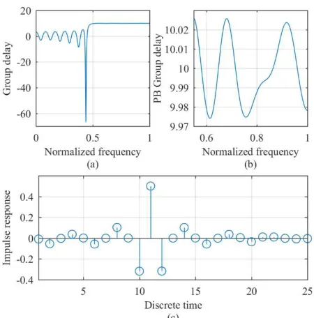
Fig. 4.4 G-FIR LP filter MM design for = 24 and group delay=10 (a) Group delay, (b) Passband group delay, (c) Impulse response………...81

Fig. 4.5 G-FIR BP filter MM design for = 24 and group delay=10 (a) Magnitude response, (b) Passband magnitude error, (c) Stopband_1 magnitude error, (d) Stopband_2 magnitude error………81

Fig. 4.6 G-FIR LP filter MM design for = 24 and group delay=10 (a) Magnitude response in dB, (b) Group delay, (c) Impulse response………..…….82

Fig. 4.7 G-FIR BS filter MM design for = 24 and group delay=10 (a) Magnitude response, (b) Passband_1 magnitude error, (c) Passband_2 magnitude error, (d) Stopband magnitude error………..…..82

(20)

xix

Fig. 4.9 G-FIR LP filter LS design for = 24 and group delay=10 (a) Magnitude response, (b) Passband magnitude error, (c) Magnitude response in dB, (d) Stopband magnitude error, (e) Impulse response, (f) Passband group delay………....85

Fig. 4.10 G-FIR HP filter LS design for = 24 and group delay=10 (a) Magnitude response, (b) Passband magnitude error, (c) Magnitude response in dB, (d) Stopband magnitude error, (e) Impulse response, (f) Passband group delay………87

Fig. 4.11 G-FIR BP filter LS design for = 24 and group delay=10 (a) Magnitude response, (b) Passband magnitude error, (c) Impulse response, (d) Stopband_1 magnitude error, (e) Passband group delay, (f) Stopband_2 magnitude error……..89

Fig. 5.1 Magnitude and group delay responses of designed lowpass filter…….…99 Fig. 5.2 Magnitude and group delay responses of designed highpass filter………100

Fig. 5.3 Convergence curve of designed lowpass filter……….100

Fig. 5.4 Convergence curve of designed highpass filter……….…101

Fig. 5.5 Magnitude and group delay responses of designed bandpass filter………...101

Fig. 5.6 Convergence curve of designed bandpass filter………102

Fig. 6.1 Discrete frequency grid points for designing 2-D circularly symmetric digital filters (Blue stands for passband; Yellow stands for stopband)………...…108

Fig. 6.2 Magnitude response of 27×27 2-D linear phase circularly symmetric FIR lowpass filter designed by TLBO………..110

Fig. 6.3 Magnitude response in dB of 27×27 2-D linear phase circularly symmetric FIR lowpass filter designed by TLBO………...110

(21)

xx

Fig.6.5 WLS error convergence curve of 27×27 2-D linear phase circularly symmetric FIR lowpass filter designed by TLBO……….………....111

Fig. 6.6 Magnitude response of 35×35 2-D circularly symmetric FIR lowpass filter designed by TLBO……….……112

Fig. 6.7 Magnitude response in dB of 35×35 2-D circularly symmetric FIR lowpass filter designed by TLBO………112

Fig. 6.8 WLS error convergence of 35×35 2-D circularly symmetric FIR lowpass filter designed by TLBO……….……..113

Fig. 6.9 Magnitude response of 39×39 2-D circularly symmetric FIR lowpass filter designed by TLBO……….…115

Fig. 6.10 Magnitude response in dB of 39×39 2-D circularly symmetric FIR lowpass filter designed by TLBO………....115

Fig. 6.11 Error convergence curve of 39×39 2-D circularly symmetric FIR lowpass filter designed by TLBO………116

Fig. 6.12 Magnitude response of 43×43 2-D circularly symmetric FIR lowpass filter designed by TLBO………...…..116

Fig.6.13 Magnitude response in dB of 43×43 2-D circularly symmetric FIR lowpass filter designed by TLBO………...….117

Fig. 6.14 Error convergence of 43×43 2-D circularly symmetric FIR lowpass filter designed by TLBO……….…117

Fig. 7.1 Cutoff frequencies of 2-d nonlinear phase FIR lowpass filters…………..123

Fig. 7.2 Magnitude response of 13×13 2-D nonlinear phase FIR lowpass filter design by TLBO……….124

(22)

xxi

Fig. 7.4 Passband group delay of 13×13 2-D nonlinear phase FIR lowpass filter design by TLBO………125

Fig. 7.5 WLS error convergence curve of 13×13 2-D nonlinear phase FIR lowpass filter design by TLBO…………...………...………..126

Fig. 7.6 Magnitude response of 15×15 2-D nonlinear phase FIR lowpass filter design by TLBO……….126

Fig. 7.7 Magnitude response in dB of 15×15 2-D nonlinear phase FIR lowpass filter design by MOTLBO……….……….127

Fig. 7.9 WLS error convergence of 15×15 2-D nonlinear phase FIR lowpass filter design by TLBO…….………128

Fig. 7.10 Magnitude response of 21×21 2-D nonlinear phase FIR lowpass filter design by TLBO………...…..128

Fig. 7.11 Magnitude response in dB of 21×21 2-D nonlinear phase FIR lowpass filter design by TLBO…………..……….….…129

Fig. 7.12 Passband group delay of 21×21 2-D nonlinear phase FIR lowpass filter design by TLBO……….…129

Fig. 7.13 WLS error convergence of 21×21 2-D nonlinear phase FIR lowpass filter design by TLBO….………...….130

Fig. 7.14 Magnitude response of 31×31 2-D nonlinear phase FIR lowpass filter design by TLBO………..……...130

(23)

xxii

(24)

xxiii

LIST OF ABBREVIATIONS/SYMBOLS

FIR Finite Impulse Response

IIR Infinite Impulse Response

TLBO Teaching-Learning-Based Optimization

MO Multiobjective Optimization

MOTLBO Multiobjective Teaching-Learning-Based Optimization

PSO Particle Swarm Optimization

MOPSO Multiobjective Particle Swarm Optimization

2-D Two-dimensional

MM Minimax

LS Least Squares

WLS Weighted Least Square

HT Hilbert Transformer

LP Lowpass

HP Highpass

BP Bandpass

BS Bandstop

PB Passband

SB Stopband

MME Maximum Magnitude Error

(25)

xxiv

GA Genetic algorithm

DE Differential Evolution

ABC Artificial Bee Colony

ACO Ant Colony Optimization

CSA Cuckoo Search Algorithm

HS Harmony Search

CSO Cat Swarm Optimization

LS-MOEA Local Search Operator Enhanced Multiobjective Evolutionary

Algorithm

MOCSO-DE Multiobjective Cat Swarm and Differential Evolution

Algorithm

(26)

1

CHAPTER 1 Introduction

Signal processing utilizes a variety of analog filters and digital filters. One

characteristic of analog signals is time-continuity, so the independent variable of a

one-dimensional analog signal is time. Through time sampling and magnitude discretization, the dimensional analog signal will be converted into a

one-dimensional discrete digital signal. Whereas, a digital filter is a system consisting

of digital multipliers, adders, and delay units. The function of a digital filter is to perform arithmetic processing on an input discrete signal to achieve the purpose of changing the signal spectrum. Therefore, designing a digital filter involves generating a transfer function that conforms a given set of specifications. In terms of hardware cost, digital filters may be more expensive than an equivalent analog filter. But from an implementation perspective, analog filters are usually built with analog components such as capacitors and inductors, where digital filters can be implemented by software or digital components. It is troublesome to replace any capacitor or inductor when the analog filter parameters are changed. Moreover, digital filters have four key advantages over analog filters [1]-[9]:

1. Digital filters are less sensitive to the external environment and have higher reliability with respect to time and temperature, unlike analog filters.

2. Digital filters enable functions such as accurate linear phase and multi-rate processing that are not possible with analog filters.

3. Digital filters can achieve arbitrary processing precision as long as the word length is increased.

4. Digital filters are more flexible and can store signals at the same time.

1.1 FIR and IIR digital filters

(27)

2

finite impulse response (FIR) and infinite impulse response (IIR) digital filters. Both have advantages and insufficiencies.

FIR filters have six key advantages over IIR filters [2]:

1. The transfer function of an FIR filter contains only zeros. An FIR filter with symmetric coefficients is guaranteed to provide a linear phase response, which can be critical in some applications.

2. Feedback is not necessary. This means that any rounding errors are not cumulative. This makes implementation simpler.

3. FIR filters are inherently stable since the output is a sum of a finite number of products of filter coefficients and input values.

4. FIR filters can easily be designed to be linear phase by making its filter coefficients symmetric.

5. FIR filters can implement linear-phase filtering. This means that the filters have no nonlinear phase shift across the frequency band. The lack of phase/delay distortion can be a critical advantage of FIR filters over IIR and analog filters in certain systems, such as digital data modems.

6. FIR filters can be used to correct frequency-response errors in a loudspeaker to a finer degree of precision than using IIR filters.

1.1.1 FIR Filters

FIR filter design can be categorized with two types: linear phase FIR filter design [24]-[28] and non-linear phase (general) FIR filter design [29]-[34]. According to the filter length M and the symmetry of impulse responses, there are four types of linear phase FIR filters [1], [5]:

(28)

3

Type I FIR filters, featured by odd M value and even symmetry, are fairly universal and most versatile, but they cannot be used whenever a 90 degrees phase shift is necessary, as is the case in differentiators and Hilbert transformers.

2. Type II Filters

Type II FIR filters, featured by even M value and even symmetry and would normally not suitable for highpass or bandstop filters because their frequency response is always 0 at = . In addition, they cannot be used for applications where a 90° phase shift is necessary.

3. Type III Filters

Type III FIR filters utilize odd M value and odd symmetry and cannot be used for standard frequency filters because, in these cases, the 90° phase shift is usually undesirable. The frequency response is always 0 at = 0 and = . They can be used for designing differentiators and Hilbert transformers.

4. Type IV Filters

Type IV FIR filters, featured by even M value and odd symmetry, cannot be used for some standard frequency-selective filters for the same reasons that type III filters cannot be used. They are well suited for differentiators and Hilbert transformers, and their magnitude approximations are usually better than type III filters because their magnitude errors are smaller. This is due to the fact that their frequency response is always 0 at = 0.

(29)

4

With the use of symmetric or asymmetric coefficients, FIR filters are guaranteed to be of linear phase. An FIR digital filter is always stable due to the absence of a denominator in its transfer function. The group delay of a linear phase FIR filter with M length is (M-1)/2, which is constant for all frequencies. This filter can always be designed as linear phase no matter its impulse responses are symmetrical or anti-symmetrical. Linear phase means that all frequency components of the input signal experience the same delay such that there are no phase distortion. For example, assuming an input signal is located within the passband of a lowpass FIR filter, and the corresponding output signal will be approximately equal to the input signal delayed by the group delay of the filter, which is just a shifted version of the input signal. Nevertheless, there is no linear phase response in a general FIR filter because the group delay is a function of frequency, the details of which will be clearer in the later chapters. The success of designing general FIR filters depends greatly on the method that is used to design their filter coefficients. In general, designing a general FIR filter to meet a set of given specification requires more computational time and a higher implementation cost.

1.1.2 IIR Filters

IIR filters are the most efficient type of digital filters with respect to implementing digital signal processing (DSP). IIR digital filters are more advantageous than FIR filters because of their implementation efficiency, which is necessary to meet specifications related to passband ripple and stopband attenuation. IIR digital filters can be designed [35]-[52] to meet the same specifications with a lower order than that of FIR digital filters. This is especially useful for implementation using a small signal processor, in which the number of calculations per time step is less than that of a FIR filter. This results in a savings of computational time.

(30)

5

of lower-order polynomials. Thus, a cascade-form digital filter can be realized as a cascade of low-order filter sections.

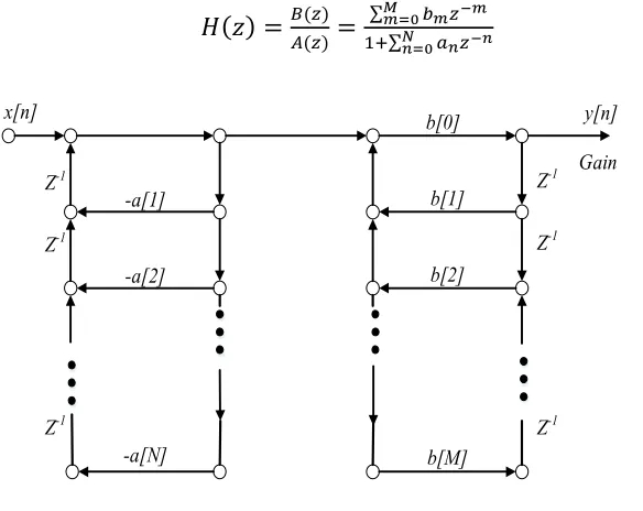
The transfer function of a direct-form IIR filter can be expressed as follows:

( ) = ( )_{( )}= ∑_∑ (1.1)

x[n] _b[0] y[n]

b[1]

b[2] -a[1]

-a[2]

-a[N] b[M]

Z-1 Gain

Z-1

Fig.1.1 Structure of direct-form I IIR digital filter

x[n] b[1] b[2] -a[1] -a[2] -a[N] b[M] y[n] b[0] Gain Z-1 Z-1 Z-1

(31)

6

The transfer function of a cascade-form IIR filter can be expressed as follows:

( ) = ∏ ( )_{( )}= ∏ ₍( )₎ (1.2)

Z-1 _Z-1

Z-1

-α11 β11

-α12

β12

β22

-α22

X Y

p0

Fig. 1.3 Structure of a cascade-form IIR digital filter (3rd_order)

Digital filters can be designed for different applications such as lowpass, highpass, bandpass, bandstop, delay equalizer, digital differentiator, digital integrator and digital Hilbert transformer. In the following chapters, different digital filter designs are described.

1.2 Two dimensional digital filters

(32)

7

processing research. Unlike a 1-D digital filter design which only involves a 1-D frequency function approximation, a 2-D digital filter design is essentially a 2-D frequency function approximation problem. The 2-D frequency function approximation theory is less developed than the 1-D frequency function approximation theory. Thus, some effective 1-D digital filter design methods cannot be extended to design a 2-D digital filter. In general, 2-D digital filter design problems are significantly more complicated than that of 1-D digital filter design problems.

(33)

8

maximally flat passband and stopband. In this context, changing filter order or flatness degree can generate various passband shapes. Additional references selected for digital filter realization and design are given in [148]-[205].

1.3 Optimization algorithms

Traditionally, numerical optimization has been the standard optimization tool [79]. In recent years, evolutionary algorithms [80] have emerged as an increasing popular optimization tool. The development of the latter was started around 1975, in which genetic algorithm (GA) [81] was proposed. The emergence and success of genetic algorithm have greatly encouraged the enthusiasm of researchers to develop nature inspired optimization algorithms. After years of development, a large number of evolutionary algorithms [80] have been developed, including genetic algorithm, ant colony optimization (ACO) algorithm, differential evolution (DE) algorithm, and particle swarm optimization (PSO) algorithm. Thus far, evolutionary algorithms have been used in a wide range of areas including machine learning, process control, economic forecasting, and engineering forecasting. The unprecedented success of evolutionary algorithms has attracted great interest from scientists in the fields of mathematics, physics, computer science, social sciences, economics, and engineering.

Swarm intelligence algorithms [82] identify questions by learning from certain life phenomena or natural phenomena. This kind of algorithm contains the characteristics of self-organization, self-learning, and self-adaptation of natural life phenomena. In the operation process, the solution space is self-organized by the obtained calculation information. In the search process, the population evolves according to the value of the fitness function set in advance by using the survival of the fittest. Consequently, the algorithm has certain intelligence. Due to the advantages of the swarm intelligence algorithms, when applying the swarm intelligence algorithm to solve a problem, it is not necessary to describe the solution problem in advance. As a result, efficient solving is possible for some complex problems.

(34)

9

population have a certain independence, and they may or may not exchange information, and their evolution mode depends entirely on their own situation. Therefore, for swarm intelligence algorithms, an individual is encapsulated in a complete and essential parallel mechanism. If a distributed multiprocessor is used to complete the process of a swarm intelligence algorithm, the algorithm can be set with multiple populations and each individual of the populations can be placed in different processors for evolution. Moreover, certain information exchanges can be completed during the iteration information, though the exchange is not necessary. After the iteration is completed, the survival of the fittest is performed according to the fitness value. Therefore, the implicit nature of the group intelligence algorithms can make full use of the multi-processor mechanism to achieve parallel programming and improve an algorithm's ability to solve problems. Thus, it is more suitable for the background of the rapid development of distributed computing technologies, such as cloud computing.

Swarm intelligence algorithms [83] are widely used to solve problems with high computational complexity, rather than trying all the options one by one, which will take a lot of time. They are used extensively in the field of artificial intelligence. For instance, the principles behind GA are borrowed from nature itself. They are the principles of heredity and variation. Genetics are the ability of organisms to pass on their biological and evolutionary characteristics to their offspring. Because of this ability, all creatures can leave their species characteristics to their offspring. The genetic variation of the organisms guarantees the genetic diversity of the population, and the variation is random because nature cannot know in advance which features are most suitable in the future due to variations on factors such as climate change, food increase/decrease, or the emergence of competitive species. Mutations cause new traits in the organism to survive and leave behind in new, changing habitats.

(35)

10

result, swarm intelligence algorithms will have problems such as premature or low solution precision. Therefore, in many cases, the barriers to solve the problem are that swarm intelligence algorithms only obtain an approximate solution to the best solution.

Swarm intelligence falls under more recent evolutionary algorithms which include differential evolution, particle swarm optimization, ant colony optimization, artificial bee colony algorithm, teaching and learning based optimization, and others. Classic evolutionary algorithms include genetic algorithms, genetic programming, and others.

1.4 Motivations of the dissertation

This dissertation concentrates on digital filter design, including FIR digital filter and IIR digital filter designs. The optimization method uses evolutionary algorithms. After experimentations and comparisons with other heuristic algorithms such as ACO, PSO, and GA, the TLBO algorithm has shown to be superior in terms of better minimization performance and faster convergence. Designing digital filters using TLBO algorithm is a new topic. Therefore, this dissertation adopts TLBO algorithm for FIR and IIR filter design.

However, when designing more complex digital filters using the TLBO, there are limitations. Therefore, improved methods are to be developed to enhance the efficiency of the TLBO algorithm. In particular, a gradient-based learning phase is proposed to replace the original learning phase to expand the search capability for digital filter design.

1.5 Organization of the dissertation

(36)

11

with crowding distance is presented. In addition, a novel multiobjective TLBO is proposed to design general FIR filters. In Chapter 5, another multiobjective is presented to design IIR digital filter. In Chapter 6, two-dimensional linear phase FIR filter design is introduced. In Chapter 7, two-dimensional nonlinear phase FIR filter using TLBO algorithm is described. In Chapter 8, future works and conclusions are presented.

1.6 Main contributions

In this dissertation, both FIR and IIR digital filter designs under least squares (LS) and minimax (MM) criteria are designed using the standard TLBO and improved algorithms. Main contributions are summarized as follows:

1. Using the standard TLBO and improved algorithms, five types of digital filters: linear phase FIR digital filters, multiobjective general FIR digital filters, multiobjective IIR digital filters, dimensional linear phase FIR filters, and two-dimensional general FIR filters are designed using minimax and least squares approximations. In general, the least squares algorithm, the Parks-McClellan algorithm, the multiobjective particle swarm optimization (MOPSO) algorithm, and others are selected for comparisons. Design results indicate improved performance can be obtained.

2. A gradient-based TLBO is developed for linear phase FIR digital filter design. Design results indicate that the gradient-based TLBO can obtain similar optimal solutions but faster convergence when compared to those of the standard TLBO.

3. A non-dominated MOTLBO with crowding distance is formed by combining the standard TLBO algorithm with non-dominated set and crowding distance. Filter design results have shown that the non-dominated MOTLBO with crowding distance can achieve faster convergence than the MOPSO in multiobjective digital filter design.

(37)

12

(38)

13

CHAPTER 2

Teaching-learning-based Optimization and Improved Algorithms

2.1 Review of swarm intelligence algorithms

Inspired by social insect behaviors, researchers have developed a series of new solutions to traditional problems through the simulation of social insects. These studies are examples of swarm intelligence research. Swarm refers to a group of subjects that can communicate directly or indirectly by changing the local environment, who can collaborate to solve distribution problems. The so-called swarm intelligence refers to the characteristics of intelligent behaviors through the cooperation of non-intelligent entities. Swarm intelligence provides the foundation for finding solutions to complex distributed problems without centralized control and without providing a global model.

The optimal solution of the swarm intelligence algorithms is the process of generating new solutions by successive iterations and evolutions of corresponding rules from random initial solutions. In swarm intelligence algorithms, the set of multiple solutions is called population, which is denoted as P(t), where P represents the size of the population (population size), and t represents the iteration. ( ),

(39)

14

In social collaboration, some individuals will be selected for information exchange and mutual learning through the corresponding selection mechanisms. The information involves four elements: (1) the method of individual selection, (2) the size of the individual, (3) the generation mechanism of the new experimental individual, and (4) the usage of the historical information of the population.

Self-adaptation mechanism refers to the individual's continuous adjustment of its status through active or passive mechanisms to adapt to the living environment in which it lives. Individuals adjust their state through global and local searches. The global search guarantees the individual's ability to explore new solutions in a wider range, which can more effectively ensure the diversity of the population and avoid premature convergence. The local search is opposite that it helps an individual to converge to the local best more easily. However, it is more effective to improve the quality of individuals by shortening the convergence of the algorithm. The self-adaptation of individuals in a population is usually used to balance the two search mechanisms. Through the above two processes, a new experimental individual can be generated.

Swarm intelligence algorithms select individuals from P parents and m

temporary sub-species into the next-generation population through a competitive mechanism. In most swarm intelligence algorithms, the size of the population is generally fixed. The individual replacement strategy is divided into the whole generation replacement strategy, r(P, m), and the partial replacement strategy,

r(P+m). The former refers to the P parents is completely replaced by the m child

generation individuals, and the latter means that only some of the P parent individuals are replaced. In order to save elite individuals, the elite retention strategy will be selected. This means that the outstanding individuals in the parent individuals are not replaced and will enter the next generation of individuals directly.

(40)

15

1. Initialize parameters such as population size and number of iterations.

2. Randomly initialize the population in the solution space.

3. While the termination condition is not met, do loop.

4. Calculate the fitness value of each individual of P(t).

5. Select some individuals for social collaborative operations.

6. Execute self-adaptation.

7. Compute competing operations to create a new generation of populations.

8. End while.

9. Output the final solution.

Through the above calculation framework, swarm intelligence algorithms apply the three operations (social collaboration, self-adaptation, and competitive evolution) to the individuals in the population. Every individual is approached the optimal solution to achieve the purpose of optimization.

PSO [86] and ACO [87] algorithms are two of the most important members of the swarm intelligence algorithm family. The basic idea is to simulate the behavior of natural biological groups to construct a stochastic optimization algorithm. The difference is that the particle swarm algorithm simulates the bird group behavior, while the ant colony algorithm simulates the ant foraging principle. These two are beneficial in this context as they are compatible with the similarities that they share, but they also complement each other due to their differences.

(41)

16

In addition, both of them are within a class of probabilistic global optimization algorithms. The advantage of the non-deterministic algorithms is that they have more chances to solve the global optimal solution. Likewise, neither is dependent on the strict mathematical nature of the optimization problem itself. The optimization process does not rely on the mathematical nature of the optimization problem itself, such as continuity, conductivity, and the mathematical description of the objective function and constraints. Both are bionic optimization algorithms based on multiple agents. Each agent in bionic optimization algorithms cooperates with each other to better adapt to the environment and demonstrates the ability to interact with the environment. Moreover, the two algorithms are intrinsic parallelism. The essential parallelism of the bionic optimization algorithm is manifested in two aspects: the inherent and intrinsic parallelism of the bionic optimization calculation. This enables bionic optimization algorithms to complete of their overall goal, which is highlighted in the movement of multiple agents' individual behaviors. Finally, both algorithms have self-organization and evolution. With memory function, all particles retain the knowledge of the solution. Thus, in an uncertain complex environment, bionic optimization algorithms can continuously improve the individual adaptability of the algorithm through self-learning.

(42)

17

convergence performance of the ant colony algorithm is sensitive to the setting of initialization parameters. In addition, ACO algorithm has a more mature convergence analysis method and can estimate the convergence speed.

As an important branch of science, swarm intelligence algorithms have been widely recognized, rapidly promoted and applied in many engineering fields, such as system control, artificial intelligence, pattern recognition, production scheduling, and computer engineering. In view of complexity, constraint, nonlinearity, multi-pole and difficult modeling of practical engineering problems, swarm intelligence algorithms are a major research target, and many researchers have sought to create an algorithm suitable for large-scale parallel and intelligent features. Since the 1980s, some novel optimization algorithms have been developed by simulating or revealing certain natural phenomena or processes. These algorithms include artificial neural networks, chaos, genetic algorithms, evolutionary programming, simulated annealing, tabu search, and hybrid optimization strategies. Collectively the novel algorithms provide new ideas and means for solving complex problems through the inclusion of mathematics, physics, biological evolution, artificial intelligence, neuroscience and statistical mechanics. For simple-function optimization problems, classical algorithms are more efficient and can obtain the exact optimal solution of the function. However, for complex-functions and combinatorial optimization problems with nonlinear and multi-extreme characteristics, classical algorithms are often unable to obtain exact optimal solutions. The unique advantages and mechanisms of these algorithms allow them to be successfully applied in many fields, thereby attracting the attention of researchers and resulting in a research boom in this field.

2.2 Literature review of TLBO algorithm

(43)

18

foragers, scouters, followers, and limits. The performance of harmony search (HS) [99]-[101] is dependent on memory consideration rate, pitch adjusting rate, and bandwidth (bw). Likewise, cuckoo search algorithm (CSA) [102]-[104] requires switching probability, step size scaling factor and Levy index. In comparison, TLBO algorithm is independent of algorithm-specific control parameters. Since TLBO algorithm was proposed, TLBO algorithm has attracted attention from researchers because of its parameter-free characteristic. In [105], TLBO algorithm was applied by manufacturing industries to solve assembly sequence problems. The TLBO algorithm was also used to design screen primer problems [106]. In [107], TLBO was used to solve optimal coordination of directional over-current relays problems. Moreover, the application of TLBO for flow shop scheduling was described in [108]-[111]. In [112], TLBO was applied to power system scheduling. Moreover, binary TLBO algorithm was used to assist for designing plasmonic nanoparticles [113].

(44)

19

(45)

20

2.3 Teaching-learning-based optimization

In TLBO algorithm, a population is composed of learners, and different design variables (or filter coefficients) are viewed as S different subjects attached to the learners. All the scores of a learner (or a solution) ( )(for = 1, 2, ⋯ , ) is evaluated collectively by the value of its objective (or error) function ( ) in an optimization problem. Within a population, the best solution is assumed to be offered and maintained by the teacher. The operations of the TLBO are divided into two phases, the teacher phase and the learner phase. In TLBO, a global search is applied to explore the starting point and then the starting point is perturbed in a local search space iteratively to arrive at an optimal solution.

1. Teacher phase

This phase is a process that a teacher teaches knowledge to the learners and improves the mean results of the class. ( ) is the mean result of the learners in a particular subject s in the tth_iteration.

( ) = ∑ , ( ) (2.1)

As the teacher is the most knowledgeable people and has the best result over all subject, let ( ) represent the teacher. Learners get knowledge from the teacher and the quality of the teacher decides the mean result, so the difference

( ) between the result of the teacher and mean result the of the learners in each subject is expressed as

( ) = × ( , ( ) − ( )) (2.2)

where , ( ) is the value of the teacher in subject s. is the teaching factor

which decides the value of mean to be changed, and rand is a random number in the range [0,1]. The value of can be either 1 or 2. The value of is decided randomly as,

(46)

21

where is not a parameter of the TLBO algorithm. The value of is not given as an input to the algorithm and its value is randomly decided by the algorithm using Eq. (2.3).

Then each learner has a potential updated counterpart and therefore

, ( ) = , ( ) + ( ) (2.4)

where ( ) is the updated value of ( )in subject s.

The algorithm accepts ( ) only if it gives a better value of objective function otherwise keeps the previous solution such that

( ) = _{( )}( ) ( ) <_{( ) ≥} ( )_{( )} (2.5)

All the accepted scores at the end of the teacher phase are maintained and these values become the input to the learner phase.

2. Learner phase

Students not only can get knowledge from the teacher but also can improve their individuals through interaction among themselves. In this step two students are randomly selected namely and ( ( ) ≠ ( )) among the entire class. After sharing or exchanging their knowledge, the new results are gained as:

( ) = ( ) + × ( ) − ( ) , [ ( )] < [ ( )] (2.6)

( ) = ( ) + × ( ) − ( ) , [ ( )] > [ ( )] (2.7)

The algorithm accepts ( ) (for = 1, 2, ⋯ , ) only if it gives a better value of objective function otherwise it keeps the previous solution such that

(47)

22

2.4 Gradient-based TLBO Algorithm

Based on analysis of previous TLBO design results, TLBO algorithm has a limitation on search ability. In order to enhance the search capability, a new phase, gradient-based phase, is proposed to improve the convergence speed and accuracy of the TLBO algorithm. The gradient descent method is a traditional method of optimization, and the gradient represents the sharpest changing trend of a function at a given point. In fact, the gradient descent method is used to numerically search for local minimum or maximum values. It is an efficient, high-speed and reliable method in practical applications.

In the gradient-based TLBO, a global search is applied to explore the starting point and then the starting point is perturbed in a local search space iteratively to arrive at an optimal solution. Moreover, a parameter—step size—is added into the gradient-based phase. A proper control parameter can improve robustness.

(48)

23

Yes No

Update by (2.12) Keep

Calculate a new score with its gradient by (2.13)

Is better than ?

Yes No

Update by (2.14) Keep

Is better than ? Keep the elite Score

(teacher )

Calculate the mean of each design variable Ms and

the new scores using (2.9) to (2.11) Initialize the population (learners), design variables (coefficients c) and termination criterion

Is the termination criteria satisfied?

Stop

Yes No

Fig. 2.1 Flowchart of gradient-based TLBO algorithm

In the gradient-based TLBO algorithm, a population is composed of learners, and different design variables (or filter coefficients) are viewed as S

different subjects attached to the learners. All the scores of a learner (or a solution)

(49)

24

Within a population, the best solution is assumed to be offered and maintained by a teacher. The operations of the gradient-based TLBO is divided into two phases, the teacher phase and the based learning phase. In the gradient-based TLBO, a search is applied to explore the starting point and then the starting point is perturbed in a local search space iteratively to arrive at an optimal solution.

1. Teacher phase

This phase is a process that a teacher teaches knowledge to the learners and improves the mean results of the class. ( ) (for = 1, 2, ⋯ , ) is the mean result of the learners in a specific subject s in the tth iteration, which is same as the teacher phase in the original TLBO algorithm. As the teacher is the most knowledge people and has the best result on that subject, let ( ) represent the teacher. Learners get knowledge from the teacher and the quality of the teacher decides the mean result, so the difference ( ) between the teacher and mean result of the learners in each subject is expressed as

( ) = ∗ ( , ( ) − ( ) ) (2.9)

where is the teaching factor which decides the value of mean to be changed, and is a random number in the range [0,1]. The value of can be either 1 or 2. The value of is decided randomly as,

= [1 + ] (2.10)

is not a parameter of the TLBO algorithm. The value of is not given as an input to the algorithm and its value is randomly decided by the algorithm using Eq. (2.10).

( )is added to current score of learners in different subjects to generate new learners:

, ( ) = , ( ) + ( ) (2.11)

(50)

25

The algorithm accepts ( ) only if it gives a better value of objective function otherwise it keeps the previous solution such that

( ) = _{( )}( ) ( ) <_{( ) ≥} ( )_{( )} (2.12)

All the accepted scores at the end of the teacher phase are maintained and these values become the input to the learner phase.

2. Gradient-based learning phase

The learner phase is not efficient due to the random selection approach in original TLBO algorithm. For this reason, a gradient-based phase is proposed to speed up the global search, which leads to (3.17)

( ) = ( ) − _{( )}( ) (2.13)

where stands for the step size.

To obtain the optimal result the score vector ( ) is selected through (2.14)

( ) = _{( )}( ) ( ) <_{( ) ≥} ( )_{( )} (2.14)

(51)

26

CHAPTER 3

Linear phase FIR filter design

Digital Hilbert transformers have many applications in the field of digital signal processing, for instance, latency analysis in neuro-physiological signals [134]; psychoacoustic design of bizarre stimuli [135]; communication problems of speech data compression [136]; multi-channel acoustic echo cancellation of regularization of convergence [137]; and auditory prostheses in signal processing [138]. Digital Hilbert transformer design can be formulated as a Type 3 and Type 4 linear phase FIR digital ﬁlter optimization problem. Both Type 3 and Type 4 linear phase FIR filters are characterized by odd symmetry. In this Chapter, a gradient-based TLBO algorithm is proposed to improve the performance of the standard TLBO algorithm. Least squares and minimax designs are used to minimize error function, several design examples of Type 3 and Type 4 Hilbert transformers using the standard TLBO algorithm and the gradient-based TLBO algorithm are presented. Design results are compared to those obtained by the least squares minimization and the Parks-McClellan algorithm [24].

In this Chapter, Section 3.1 describes the formulation of Hilbert transformer design problem and objective functions; Section 3.2 presents the design examples and results; Section 3.2.1 shows the Type 3 bandpass HT designs; Section 3.2.2 describes Type 4 highpass HT designs; Section 3.2.3 provides a comparison with least squares algorithm and minimax algorithm; and Section 3.3 gives conclusions.

3.1 Problem formulation

3.1.1 Type 3 Linear Phase FIR Digital Filters

The causal transfer function of an M odd and odd symmetry FIR digital filter can be expressed [1] as

(52)

27

where ℎ( ) for = 0to ( − 1)/2 represent the unique set of impulse responses.

According to the M odd and odd symmetrical features of the Type 3 linear phase Hilbert transformer, the coefficient vector h is given by

= [ℎ(0), ℎ(1), ℎ(2), ⋯ , ℎ( ), ⋯ , ℎ( − 2), ℎ( − 1)] (3.2)

ℎ( ) = −ℎ( − 1 − ) for 0,1,2,3, ⋯ , (3.3)

The frequency response can be evaluated by substituting = into (3.1) as

( ) = ∑( )2ℎ( ) sin − (3.4)

The N (=M-1)th-order Type 3 linear phase digital Hilbert transformer can be

represented by

( ) = ( , ) (3.5)

where

( , ) = ( ) (3.6)

= , , , … , (3.7)

= 2 ℎ _{2 − 1 , ⋯ , ℎ(2), ℎ(1), ℎ(0)}− 1

= ℎ = 0 (3.8)

( ) = sin( ) sin(2 ) ⋯ sin (3.9)

From (3.4), the term j corresponds to / _{, the group delay response of the}

(53)

28

( ) = − ( ) = − = (3.10)

3.1.2 Type 4 Linear Phase FIR Digital Filters

The transfer function of a causal M even and odd symmetry linear FIR digital filter [1] is given by

( ) = ∑ ℎ( ) 1 − [ ( )] _(3.11)

The Type 4 linear phase digital Hilbert transformer is (= + 1) even and odd symmetry such that its impulse responses can be expressed as

= [ℎ(0), ℎ(1), ℎ(2), … , ℎ( ), … , ℎ( − 2), ℎ( − 1)] (3.12)

ℎ( ) = −ℎ( − 1 − ) for = 0,1, 2, 3, … , − 1 (3.13)

The frequency response of a Type 4 linear phase digital Hilbert transformer can be evaluated by substituting = into (3.11) as

( ) = ∑ 2ℎ( ) sin − = ( , ) (3.14)

where

( , ) = ( ) (3.15)

= , , , , … , = 2 ℎ − 1 , ⋯ , ℎ(2), ℎ(1), ℎ(0) (3.16)

( ) = sin( ) sin ⋯ sin (3.17)

From (3.14), the term j corresponds to / _{, the group delay response of the}

odd Nth-order Type 4 linear phase digital Hilbert transform is

(54)

29

3.1.3 Hilbert Transformer

The ideal frequency response of a digital Hilbert transformer is denoted as (3.19) in [80

( ) = − for 0 ≤ ≤ (3.19)

where the parameter denotes the group delay. The frequency response ( ) is related to the desired amplitude response ( ) by

( ) = ( ) = (−1)

for 0 ≤ ≤ (3.20)

According to (3.20), the ideal amplitude response of the digital Hilbert transformer is defined by

( ) = −1 for 0 ≤ ≤ (3.21)

3.1.4 Objective Functions

3.1.4.1 Minimax design

The optimization problem for Type 3 and Type 4 Hilbert transformer is to search for an optimal coefficient vector that minimizes the weighted minimax (MM) objective function ( ) with respect to as defined [1] by

min ( ) = min[∑ ( )| ( , ) − ( )| ] /

for ∈ (3.22)

where is the optimization frequency grid; and is even.

For simplicity, the amplitude response is considered, the weighted minimax function ( ) is expressed by

min ( ) = min[∑ ( )| ( , ) − ( )| ] /

for ∈ (3.23)

(55)

30

The optimization problem both for Type 3 and Type 4 Hilbert transformer is to search for an optimal coefficient vector that minimizes the weighted least square (LS) objective function ( ) with respect to as defined [1] by

min ( ) = min[∑ ( )| ( , ) − ( )| ]

for ∈ (3.24)

3.2 Designs and Results

In this chapter, Type 3 linear phase FIR bandpass digital Hilbert transformers of orders N=14, 26, 38 and 50 and Type 4 linear phase FIR highpass digital Hilbert transformers [1] of orders N=13, 25, 37 and 49 are designed using the standard TLBO algorithm for MM design, as well as the standard TLBO algorithm and the gradient-based TLBO algorithm for LS design.

The initialization of filter coefficients is obtained by adding ±random values to the filter coefficient values obtained by the Matlab function firpm.m for MM designs and by the Matlab function firls.m for LS designs to ensure all the coefficients are within the bound limits.

3.2.1 Type 3 bandpass HT MM designs

(56)

31

Table 3.1 FIR Filter and TLBO (Gradient-based TLBO) Parameters (Key: LP-FIR 3: Type 3 FIR Hilbert transformer)

Symbol Description Value

( ) Frequency weights for 0 ≤ ≤ 1

[ ] _{Upper bound of filter coefficients} _0.94 [ ] _{Lower bound of filter coefficients} _-0.94

Gradient-based TLBO population size 14 26 38 50 Order of LP-FIR3 filter 14 26 38 50 Number of distinct coefficients of LP-FIR3 filter 7 13 19 25 Group delay of LP-FIR3 filter 7 13 19 25

Table 3.2 Frequency Grid and Desired Amplitude Response

N Frequency Grid ( )

Optimization

14 [0.10:0.005:0.90] [21:181] 26 [0.08:0.005:0.92] [17:185] 38 [0.06:0.005:0.94] [13:189] 50 [0.04:0.005:0.96] [9:173]

Evaluation

14 [0.10:0.001:0.90] [101:901] 26 [0.08:0.001:0.92] [81:921] 38 [0.06:0.001:0.94] [61:941] 50 [0.04:0.001:0.96] [41:961]

Table 3.3 Hilbert transformer minimax errors (Keys: : Type; BP: Bandpass; HP: Highpass; : Filter order; : Algorithm; 1: firpm.m; 2: TLBO; CPU: Time in sec)

Minimax error Iteration CPU

3 BP

14 1 0.063859638428037 _{2 0.048437168979108} _2,500- 0.11 _1.14 26 1 0.056149417077486 _{2 0.014541694349349} _7,500- 0.10 _6.86

38 1 0.050680262166871 _{2 0.010494629986522} _7,500- 0.14 _9.57

(57)

32

Table 3.4 Hilbert transformer minimax peak error (Keys: : Type; BP: Bandpass; : filter order; MM: Minimax; : Algorithm; 1: firpm.m; 2: TLBO; : Peak error

frequency; C: Converged iteration number)

Peak MM error

3 BP

14 1 0.062508534703398 0.282 _{2 0.047738450350362 0.147} ₂₂₆-

26 1 0.055209896344805 0.814 _{2 0.014405922412530 0.101} _1,679-

38 1 0.049964067125621 0.494 _{2 0.010421858229430 0.893} _1,668- 50 1 0.057192424608021 0.743 _{2 0.017715320356500 0.520 1,826,795}-

(58)

33

Fig. 3.2 Convergence curve of minimax error for Hilbert transformer design for Type 3 N =14 (a) Interval 1, (b) Interval 2

(59)

34

(60)