Improving Adaptive Video Streaming through Machine Learning

University of Windsor University of Windsor

Scholarship at UWindsor

Scholarship at UWindsor

Electronic Theses and Dissertations Theses, Dissertations, and Major Papers

2018

Improving Adaptive Video Streaming through Machine Learning

Improving Adaptive Video Streaming through Machine Learning

Anh Minh Le

University of Windsor

Follow this and additional works at: https://scholar.uwindsor.ca/etd

Recommended Citation Recommended Citation

Le, Anh Minh, "Improving Adaptive Video Streaming through Machine Learning" (2018). Electronic Theses and Dissertations. 7373.

https://scholar.uwindsor.ca/etd/7373

This online database contains the full-text of PhD dissertations and Masters’ theses of University of Windsor students from 1954 forward. These documents are made available for personal study and research purposes only, in accordance with the Canadian Copyright Act and the Creative Commons license—CC BY-NC-ND (Attribution, Non-Commercial, No Derivative Works). Under this license, works must always be attributed to the copyright holder (original author), cannot be used for any commercial purposes, and may not be altered. Any other use would require the permission of the copyright holder. Students may inquire about withdrawing their dissertation and/or thesis from this database. For additional inquiries, please contact the repository administrator via email

Improving Adaptive Video Streaming through Machine Learning

By

Anh Minh Le

A Thesis

Submitted to the Faculty of Graduate Studies

through the School of Computer Science

in Partial Fulfillment of the Requirements for

the Degree of Master of Science

at the University of Windsor

Windsor, Ontario, Canada

2017

Improving Adaptive Video Streaming through Machine Learning

by

Anh Minh Le

APPROVED BY:

______________________________________________

S. Nkurunziza

Department of Mathematics and Statistics

______________________________________________

S. Mavromoustakos

School of Computer Science

______________________________________________

J. Chen, Advisor

School of Computer Science

iii

DECLARATION OF ORIGINALITY

I hereby certify that I am the sole author of this thesis and that no part of this

thesis has been published or submitted for publication.

I certify that, to the best of my knowledge, my thesis does not infringe upon

anyone’s copyright nor violate any proprietary rights and that any ideas, techniques,

quotations, or any other material from the work of other people included in my

thesis, published or otherwise, are fully acknowledged in accordance with the

standard referencing practices. Furthermore, to the extent that I have included

copyrighted material that surpasses the bounds of fair dealing within the meaning of

the Canada Copyright Act, I certify that I have obtained a written permission from

the copyright owner(s) to include such material(s) in my thesis and have included

copies of such copyright clearances to my appendix.

I declare that this is a true copy of my thesis, including any final revisions,

as approved by my thesis committee and the Graduate Studies office, and that this

thesis has not been submitted for a higher degree to any other University or

iv

ABSTRACT

While the internet video is gaining increasing popularity and soaring to

dominate the network traffic, extensive study is being carried out on how to achieve

higher Quality of Experience (QoE) in its content delivery. Associated with the

HTTP chunk-based streaming protocol, the Adaptive Bitrate (ABR) algorithms have

recently emerged to cope with the diverse and fluctuating network conditions by

dynamically adjusting bitrates for future chunks. This inevitably involves predicting

the future throughput of a video session. Predicting parameters being part of the

ABR design, we propose to follow the data-driven approach to learn the best setting

of these parameters from the study of the backlogged throughput traces of previous

video sessions. To further improved the quality of the prediction, we propose to

follow the Decision Tree approach to properly classify the logged sessions according

to those critical features that affect the network conditions, e.g. Internet Service

Provider (ISP), geographical location etc. Given that the splitting criterion will have

to be defined together with the selection among ABR parameter values, existing

Decision Tree solutions cannot be directly applied. In this thesis, some existing

Decision Tree algorithm has been properly tailored to help learning the best

parameter values and the performance of the ABRs with the learnt parameter values

is evaluated in comparison with the existing results in the literature. The experiment

shows that this approach can improve the performance of an ABR algorithm by up

to 8.59%, with 98.38% of the testing sessions performing better than having a fixed

v

ACKNOWLEDGEMENTS

I would like to acknowledge and say my thanks to the following people who have

supported me throughout the time I study in the Master program in University of

Windsor.

Firstly, I would like to express my gratitude to my advisor Dr. Jessica Chen, for

her unwavering support, guidance and insight throughout this research paper. I

would also like to thank her for pointing out my weak point so I can continue to

improve myself.

Secondly, I would like to thank Dr. Sévérien Nkurunziza and Dr. Stephanos

Mavromoustakos for accepting the part of being my external and internal reader

and for their help on pointing out the mistake I made during my proposal so I can

finally deliver this thesis successfully, as well as Ms. Karen Bourdeau for helping

me throughout the process of taking this Master program.

And finally, I would like to thank all my friends and family for their unwavering

support and encouragement. You have all give me the confident and support I need

vi

TABLE OF CONTENTS

DECLARATION OF ORIGINALITY ... iii

ABSTRACT ... iv

ACKNOWLEDGEMENTS ... v

LIST OF ABBREVIATIONS/SYMBOLS ... vii

CHAPTER 1 INTRODUCTION ... 1

CHAPTER 2 PRELIMINARY WORK ... 2

2.1/ Video Streaming, how does it work? ... 2

2.2/ Related Work ... 3

CHAPTER 3 PROBLEM STATEMENT, SOLUTION AND ALGORITHM ... 7

3.1/ Problem Statement ... 7

3.2/ BBA algorithm ... 8

3.3/ Comparing parameters set ... 11

3.4/ Decision Tree Training ... 14

3.5/ Decision Tree Testing ... 18

CHAPTER 4 DATASET, TESTING RESULT AND CONCLUSION ... 19

4.1/ Dataset ... 19

4.2/ Testing Result ... 20

4.3/ Future Work ... 33

4.4/ Conclusion ... 34

REFERENCES/BIBLIOGRAPHY... 35

vii

LIST OF ABBREVIATIONS/SYMBOLS

QoE

Quality of Experience

ABR

Adaptive Bitrate

ISP

Internet Service Provider

VOD

Video-on-demand

BBA

Buffer Based Algorithm

AI

Artificial Intelligence

Geolocation

Geographical Location

1

CHAPTER 1

INTRODUCTION

Live Streaming and video-on-demand (VOD) are becoming the most popular methods to watch videos as the internet expands and gets more and more accustomed to our daily life. It was estimated that the entire video streaming market is worth of around US$30.29 billion in 2016, and will grow up to US$70.05 billion by 2021[1]. Youtube, with one of the most popular video streaming platform, reported that the consumption rate of mobile videos is rising 100% every year. Netflix reported that 10 billion hours of video was watched per month by its user base [2].

In this growing market with a large number of competitors, improving Quality of Experience (QoE) for the users when they watch videos is a key factor for any publisher who wants to attract and retain its customers. From Livestream and New York Magazine’s survey [2], video quality was the most important factor for 67% viewers when they watch a livestream broadcast, and about 62% consumers are more likely to have a negative perception of a brand name of a company who has the video content delivered with low-quality.

It is, however, not an easy task to improve video quality, because there are many factors that contribute to the users viewing experience. According to a survey by JWplayer in 2016, the users are considering many factors that affect their QoE with a streaming service, with 24% considering that re-buffering ratio is the most important factor of their experience, and about 12% thinking that average bit rate, which is linked directly to the quality of a video, is the most important part, and another 12% saying that the most important factor is the time for a video to get started [3].

2

CHAPTER 2

PRELIMINARY WORK

In order to better explain the ultimate goal of the present thesis, first we introduce the key terminologies and give a brief introduction on how video streaming works. Then we will give a brief overview of recent approaches to improving the QoE of the video viewers.

2.1/ Video Streaming, how does it work?

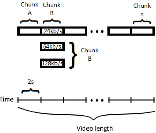
Video Streaming, by definition, is the act of streaming a video over the internet from a server to the user. From a more technical perspective, it is a constant data stream of a video kept downloaded to the user’s device until either the data has been completely downloaded or the user has stopped watching. With the internet growing and video streaming getting more popular, many techniques have been developed in order to bring the best video streaming quality to different users. Video content now are usually partitioned into small chunks of a few seconds each [4]. Each chunk has many different versions stored on the server, encoded with different bitrates. The bitrate is essentially the amount of data per second played on a video device. The higher the bitrate of a chunk is, the higher the quality of that chunk can be displayed to the user.

3

The purpose of partitioning a video file into chunks like this is to make it easier to dynamically switch among different bitrates during a video streaming session. The necessity of switching among different bitrates on the go came from the fact that the internet download speed does not stay constant throughout an entire viewing session, which is defined by the period from the time the user starts watching a video to the time he/she stops watching it.

While a player can download in a second more than a second of video data, within that same time, the user will only be able to watch one second of the video. Hence, all the chunks downloaded but not yet played are saved in a buffer on the client side. Buffer size is the maximum amount of data or video chunks a client can hold at a time. It can be calculated using either the number of bytes or the number of seconds. We consider the model where a video player will not start playing a chunk until it has been completely downloaded, and will not download the next chunk until a space big enough for an entire chunk is available in the buffer.

In regard to the user experience, there are some terminologies that need to be explained [5]. The first one is start time, or join time, which is the period from the time when the user clicks on a video for viewing, to the time when the user actually starts watching the video. Usually this amount of time is used for the play buffer to get loaded with a few initial chunks. From the user’s viewpoint, the lower this time is, the better. The second is re-buffering time, which is the total amount of time the video gets stopped or frozen in the middle of a playing session when the play buffer becomes empty, and the viewer has to wait for the player to download a new chunk of video. Similar to join time, the less this occurs, the better. The third is average bitrate, which is the average of the bitrates of all the chunks in a video downloaded over an entire viewing session. This value indicates overall how good the video display quality is, and the higher this value is, the better. In addition to these three attributes that can be used to determine the QoE, there are some other QoE metrics, for example: the number of times re-buffering happens, the number of times bitrate changes etc. Each ABR algorithm is designed with a different focus on different aspects of QoE, so there’s no universal unique formula to define QoE. For the purpose of this thesis, we will mainly consider join time, re-buffering, and average bitrate.

2.2/ Related Work

4

condition while viewing a low bitrate video, ABR algorithms will try to increase the bitrate of that video.

There exist many different approaches to ABR algorithms. In An Optimized Stall-Cautious Adaptive Bitrate Streaming Algorithm for Mobile Network [6], the author divided ABR algorithms into three main classes: rate-based algorithms, buffer-based algorithms and optimized streaming algorithms. For rate-based class, ELASTIC [7] is a good example. ELASTIC is a client-side algorithm using feedback control theory to construct a single controller that will throttle the video level (bitrate) to fill up the buffer to a set buffer length to ensure the video playback will not have re-buffering. In its formula for the controller:

q(t) and qI(t) are different states of the buffer, and kp and ki are 2 parameters of the controllers that are set to 0.01 and 0.001 respectively by default as proposed by the author of this paper.

For buffer-based class, we have Buffer Base Algorithm (BBA) [8] which uses the buffer state of the client’s video player to choose the bitrate of the video. BBA proposed to set up a few parameters: the reservoir, upper reservoir and an f(B) function which determines the relationship between the bitrate and the buffer state in this algorithm (see figure 2.2).

Figure 2.2: Buffer Base Algorithm model

5

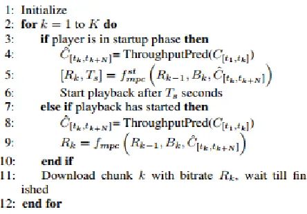
In the optimized streaming algorithm class, we have MPC algorithm [9]:

Figure 2.3: Video adaptation workflow using MPC

which is based on the assumption that network condition should be reasonably stable and do not change too drastically within a short period of time. With that assumption, we can try to look N steps ahead and solve a specific QoE maximization problem. Within this algorithm, the look-ahead window N is a parameter that can be changed to suit each individual user better. It’s worth noting that in this case, while a larger window size N is usually better, it will also negatively impact the runtime of the algorithm thus making the algorithm not being able to work efficiently at runtime. It’s also worth noting that through the research reported in CS2P [10], we know that some key features such as ISP and geographical locations do have serious impacts on the network condition of a client, and thus can be used to improve the ABR performance on future sessions.

6

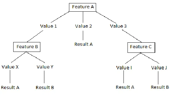
Figure 2.4: Decision Tree example

There are different approaches to constructing Decision Trees, including binary split, where at each node, the tree can only be split into two branches, and multi-way split, where at each node, the tree can be split into as many branches as the number of values the chosen feature has [13]. A feature chosen to be a splitting criteria usually is determined based on how much information gain can be obtained by choosing the considered feature to split the current node. There are also different approaches to dealing with the data that was not present in the decision tree, with the two popular approaches: (i) the technique used in C4.5[14]by putting the new value into all the branches and give each vote from each branch a weight based on how many instances are present in that branch. For example, if we have 2 branches with 100 instances and 50 instances respectively, the vote got from going down the 1st branch will be given a weight of 1/1.5, while the vote got from going down the 2nd branch will be given a weight of 0.5/1.5. (ii) the technique used in CART [15] by putting the new value into the branch with the most number of instances [16].

7

CHAPTER 3

PROBLEM STATEMENT, SOLUTION AND ALGORITHM

3.1/ Problem Statement

Having reviewed different ABR algorithms and techniques used to improve QoE, we come to the realization that the parameters in each algorithm are usually fixed by the authors based on testing the algorithm on a large set of data with different user cases and choosing a set of parameters that fit well with the users in general. However, it is easy to see that not all users have the same viewing condition. Different users have different internet conditions affecting their video viewing experience in many ways, leading to some having a vastly different viewing experience compare to others who watch the same video on the same server. From the study in CS2P, we learned that the key factors that impact the user’s viewing experience are the user’s conditions such as ISP, geographical location, and device model.

Stemmed from that observations, we can easily see that: should we want the existing ABR algorithms to serve the user in a better way, the algorithm itself should be adapted to each user cases. To do that manually is inefficient, so we turn to Machine Learning for help with this problem. With Machine Learning, the computer itself can learn what kind of parameters are most suitable for each user and adjust the algorithm accordingly. The key issue here is that in many classes, we have a wide variety of possible values. For example, for ISP, we have Bell, AT&T, Verizon etc. We choose to use Decision Tree in order to quickly go through a new user’s setting and retrieve the suitable parameters setting based on previously learned user cases. However, we cannot directly apply the Decision Tree algorithms, due to the following major issues:

● Decision Tree is usually used for classification problem with only two classes: true and false, and in our case, while we can call our problem classification, the parameters set we have are not limited to two.

● The best parameters set for each node and leaf can change when a node is split. So, we will need to modify the Decision Tree algorithm to best suit our need for this case. In this chapter, we will look more into the problem with the normal Decision Tree algorithm and how we make a modification to it.

8

3.2/ BBA algorithm

BBA algorithm, proposed by Te-Yuan Huang, Ramesh Johari, Nick McKeown, Matthew Trunnell and Mark Watson, is a result of collaboration research between Stanford University and Netflix Inc. to develop an ABR algorithm that depends solely on the buffer condition on the client side to dynamically change the video bitrate for a better QoE for the users of Netflix. The idea of the algorithm is very simple: with a predefined setting of the 3 parameters, i.e. reservoir, upper reservoir and an f(B) function which define the cushion area, the ABR algorithm will then only need to look at where the current value of the buffer fits into the predefined setting, and set the bitrate for the next video chunk accordingly as shown in figure 2.2.

In the 1st _{iteration of this BBA0 algorithm, as the algorithm was designed with a long video} viewing sessions in the Netflix platform in mind, the buffer size is also set to a very large value of 240 seconds, with the reservoir size set to 90 seconds, cushion from 90 to 216 seconds, and the upper reservoir 216 to 240 seconds. In other words, the reservoir size is 37.5%, upper reservoir is 10%, and the rest is for cushion. For example, when the buffer has only 40 seconds of video left, the BBA algorithm will set the bitrate of the next video chunk to the minimum available bitrate; when there are 220 seconds of video currently downloaded in the buffer, the algorithm will keep the bitrate to the maximum; when the buffer length is between 90 to 216, the algorithm uses function f(B) to calculate a suitable bitrate value accordingly.

Now let us consider what will happen when we change the parameters of this algorithm. If the reservoir is set to a bigger size, the ABR will prefer the bitrate to be at minimum, which will definitely help dealing with the re-buffering problem, but will also make the average bitrate of the video relatively low. For the f(B) function, if the slope is too high, the bitrate will fluctuate too much with even a slight change in the buffer. The algorithm prefers the maximum bitrate, which, while increasing the overall average bitrate of the video sessions, will more likely to increase re-buffering time. If the slope is too low, it may decrease the average bitrate of the video sessions and the ABR will not respond to the change in the buffer fast enough.

9

We have followed the BBA0 algorithm on backlogged traces in the data set to get the average bitrate and rebuffering ratio of each session. But with multiple QoE metrics, it is hard to tell directly how each session performs compared to others, so we will be converting those values into a single QoE value. As stated in chapter 2, there is no predefined unique QoE calculation formula. As such, in this thesis, we will be using QoE formula defined in the following way:

𝑄𝑜𝐸(𝑟, 𝑠, 𝑝) =𝑟 ∗ 𝑟𝑒𝑏𝑢𝑓𝑅𝑎𝑡𝑖𝑜(𝑠, 𝑝) + 1 𝐴𝑣𝑔𝐵𝑖𝑡𝑅𝑎𝑡𝑒𝑅𝑎𝑡𝑖𝑜(𝑠, 𝑝)

Here r is the weight of the rebufRatio, set to 20 by default. This weight r is used to express how much we want to emphasis on the rebuffering in our QoE formula. Should we want the rebuffering to have a larger role, we increase r, and should we want the rebuffering to be considered with less priority, we decrease r. s is session id. p is the parameter value used in the BBA0 algorithm to calculate this QoE. AvgBitRateRatio(s,p) is the average bitrate of session s with parameter value p over the maximum bitrate available. For example, if the AvgBitRate is 2300kb/s and the maximum possible bitrate is 2500kb/s, AvgBitRateRatio will be 2300/2500 or 0.92. The rebufRatio(s,p) is the rebuffering Ratio of session s with parameter value p. With this formula, the lower the QoE, the better, as QoE will decrease as the AvgBitRateRatio rises, and increase as the rebuffering ratio rises.

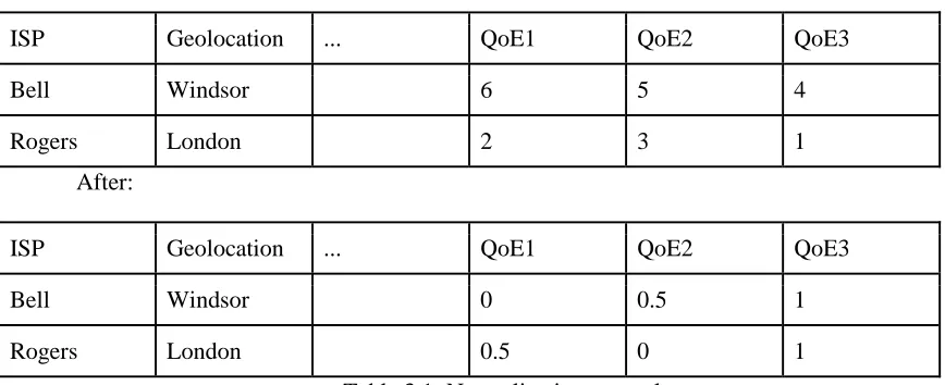
With the baseline of how BBA0 performs, we can now move on to change the parameters of the BBA algorithm, in order to see how such changes affect the algorithm. There are two parameters we can change: the reservoir and the slope. The change in either one will give us a different QoE value. So, we can have a table of QoE values from different parameter sets. It’s worth noting that for some session with a low throughput rate, it will yield a lower QoE value no matter what parameter value is chosen. In order to have the QoE values comparable among all sessions, we normalize the results by using the normalization formula below, and Table 3.1 shows some sample results.

𝑛𝑜𝑟𝑚𝑄𝑜𝐸(𝑟, 𝑠, 𝑝) = 1 − 𝑄𝑜𝐸(𝑟, 𝑠, 𝑝) − min⁡{𝑄𝑜𝐸(𝑟, 𝑠, 𝑝𝑖)|𝑝𝑖 ∈ 𝑃} max{𝑄𝑜𝐸(𝑟, 𝑠, 𝑝𝑖)|𝑝𝑖 ∈ 𝑃} − ⁡min⁡{𝑄𝑜𝐸(𝑟, 𝑠, 𝑝𝑖)|𝑝𝑖 ∈ 𝑃}

10

Before:

ISP Geolocation ... QoE1 QoE2 QoE3

Bell Windsor 6 5 4

Rogers London 2 3 1

After:

ISP Geolocation ... QoE1 QoE2 QoE3

Bell Windsor 0 0.5 1

Rogers London 0.5 0 1

Table 3.1: Normalization example

Now with all the QoE values normalized, we need a way to compare QoE result from one parameter set with the one from another parameter set. The way we choose to do this is to take average QoE of all the sessions obtained from applying this parameter set, using normQoE formula. With that, we can know which one is the best QoE set currently. The reason why we need to know this is that this would be the parameter set that would be chosen when we want to select a parameter value for the entire user base as it gives the best QoE value according to our QoE formula. More details about this will be given in chapter 3.3. The best parameter set calculated from this method will be used as our base value to compare with the result we obtained after running Machine Learning in order to see how much Machine Learning can improve this value even further.

𝑄𝑜𝐸(𝑟, 𝑆, 𝑝) = ⁡ 1

|𝑆|∑ 𝑄𝑜𝐸(𝑟, 𝑠, 𝑝)

𝑠∈𝑆

𝑆𝑖𝑛𝑔𝑙𝑒𝐵𝑒𝑠𝑡𝑄𝑜𝐸(𝑟, 𝑆) = max⁡{𝑄𝑜𝐸(𝑟, 𝑆, 𝑝𝑖)|⁡𝑝𝑖 ∈ 𝑃}

𝑛𝑜𝑟𝑚𝑄𝑜𝐸(𝑟, 𝑆, 𝑝) = ⁡ 1

|𝑆|∑ 𝑛𝑜𝑟𝑚𝑄𝑜𝐸(𝑟, 𝑠, 𝑝)

𝑠∈𝑆

𝑆𝑖𝑛𝑔𝑙𝑒𝐵𝑒𝑠𝑡𝑁𝑜𝑟𝑚𝑄𝑜𝐸(𝑟, 𝑆) = max⁡{𝑛𝑜𝑟𝑚𝑄𝑜𝐸(𝑟, 𝑆, 𝑝𝑖)|⁡𝑝𝑖 ∈ 𝑃}

11

3.3/ Comparing parameters set

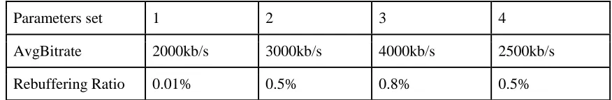
For the first part of this thesis, we want to propose a way to systematically compare different parameters set to each other. As stated in the previous section, for our testing, we are only looking to compare the average bitrate and rebuffering ratio between each data set comprised from different parameters set. We can then obtain a table of data of different parameters set with different results that will look like table 3.2:

Parameters set 1 2 3 4

AvgBitrate 2000kb/s 3000kb/s 4000kb/s 2500kb/s

Rebuffering Ratio 0.01% 0.5% 0.8% 0.5% Table 3.2: Comparing parameters set

Through some initial testing, we found out that with different parameters set being tested, usually what we obtain is a tradeoff between average bitrate and rebuffering ratio, because when average bitrate goes up, the rebuffering ratio usually goes down, and vice versa. So with that observation, it is difficult to say that one parameters set is better than every other set unless both the average bitrate and rebuffering ratio get improved. As the higher the average bitrate the better, and the lower the rebuffering ratio the better, we can define that a parameters set i producing the result avgBitratei and rebufi is better than parameters set j that produces the result avgBitratej and rebufjif and only if avgBitratei >= avgBitratei and rebufi<= rebufj.

(𝑎𝑣𝑔𝐵𝑖𝑡𝑟𝑎𝑡𝑒_𝑖, 𝑟𝑒𝑏𝑢𝑓𝑖) ≥ ⁡ (𝑎𝑣𝑔𝐵𝑖𝑡𝑟𝑎𝑡𝑒𝑗, 𝑟𝑒𝑏𝑢𝑓𝑗)

<=> 𝑎𝑣𝑔𝐵𝑖𝑡𝑟𝑎𝑡𝑒𝑖 ≥ 𝑎𝑣𝑔𝐵𝑖𝑡𝑟𝑎𝑡𝑒𝑗⁡&&⁡𝑟𝑒𝑏𝑢𝑓𝑖≤ 𝑟𝑒𝑏𝑢𝑓𝑗

12

single best parameters set that is suitable to our need and that will perform better than other parameters sets according to our QoE formula.

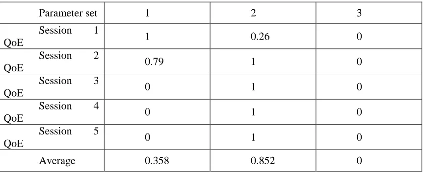
One example of another factor that can change the definition of single best parameters set is the way we normalize the data. What we are doing right now is local normalization where we normalized the data within each session (locally), but on the other hand, we also have global normalization. Global normalization works by taking into consideration the entire data set instead of just within each session. For example, consider the following table 3.3:

Parameter set 1 2 3

Session 1

QoE 1 15 20

Session 2

QoE 5 1 20

Session 3

QoE 20 19 20

Session 4

QoE 20 19 20

Session 5

QoE 20 19 20

Total 66 73 100

Table 3.3: Example data set (Lower is better)

If we were to use local globalization, the best parameters set will be set 2 as after local normalization, we have the result look like this:

Parameter set 1 2 3

Session 1

QoE 1 0.26 0

Session 2

QoE 0.79 1 0

Session 3

QoE 0 1 0

Session 4

QoE 0 1 0

Session 5

QoE 0 1 0

Average 0.358 0.852 0

13

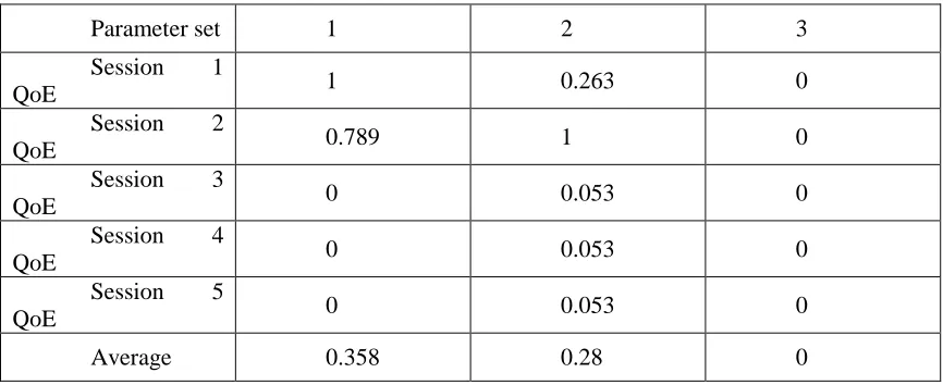
With this, we can see that parameters set 2 is the best one as most of the sessions prefer set 2. However, if we were to use global normalization, we got table 3.5:

Parameter set 1 2 3

Session 1

QoE 1 0.263 0

Session 2

QoE 0.789 1 0

Session 3

QoE 0 0.053 0

Session 4

QoE 0 0.053 0

Session 5

QoE 0 0.053 0

Average 0.358 0.28 0

Table 3.5: Global normalization (Higher is better)

With this, parameters set 1 become the best one instead of parameters set 2. But as we have talked about in this chapter, global normalization and local normalization are just other ways to define a different single best parameters set, which comes with its own tradeoff. Global normalization focuses more on the betterment of the overall average QoE, and is willing to sacrifice/allow more sessions to have worse QoE as long as the total average QoE increases, while local normalization focuses more on the betterment of the number of sessions that perform better, and is willing to sacrifice/allow the overall average bitrate to become worse. If we think about it in term of the user, global normalization allows for the happy customers to become happier at the cost of more unhappy customers, while local normalization allows for more happy customers to exist at the cost of the already happy customers become slightly less happy. So local and global normalization therefore are just different ways to choose the best QoE. Out of the two, we choose to go with local normalization for our testing as our goal with the decision tree is more in line with the advantage that local normalization offers.

14

3.4/ Decision Tree Training

First, let’s recap on how normal Decision Tree works. Decision Tree is used to classify data, usually into two groups per step, each of them being a class, which is defined based on a training data set provided. From the root of the tree, which is the node that contains all the training data set, the Decision Tree algorithm will go over all the features of that dataset and try to find which feature is the best to be used to split the data set into two (for binary split) or multiple subsets (for multiway split). The way Decision Tree algorithm defines the best feature is according to which feature gives the best information gain across all the split sets, or in other word, lowest entropy among all the split sets. Here, entropy is a measure of the randomness in the information being processed [17], or we can call it the impurity of a dataset.

𝐸𝑛𝑡𝑟𝑜𝑝𝑦 = ⁡ − ∑ 𝑝𝑖 𝑖

(𝑙𝑜𝑔2𝑝𝑖)

That’s how a normal classification decision tree works, but in case the response are continuous values instead of categorical ones, we also have another subclass of decision tree called Regression Tree, which splits the data according to the minimum Mean Squared Error of the child nodes after being split by a feature.

𝑀𝑆𝐸 = ⁡1

𝑁∑(𝑦 − 𝑦𝑖)

2 𝑁

𝑖=1

When a data set is split, if a split child has most of its data belonging to a same class, the entropy of the said child will be low. Thus, the information gain is high, and the feature is preferred over other available features. The tree will stop splitting once one of the stopping criteria is meet. These include: (i) the number of instances in a node is too small; (ii) the depth of the tree is too high; and (iii) all values of all child nodes are of the same class. Once a full tree was constructed this way, the Decision Tree can aid in the process of classifying a new data to determine whether it belongs to this class or the other by going down the tree with the feature of the new data. Should the new data that are being classified have a feature value not used or are new to the decision tree, there are two popular approaches to this, either (1) put all new data down to the child node with the highest number of instances, which is used in CART; or (2) put the new data down to all the child nodes with a weight proportional to the number of instances of each child, which is used in C4.5. CART and C4.5 are two popular decision tree algorithms.

15

Session ISP Country City Device Model

OS QoE1 QoE2 QoE3

1 Bell Canada Windsor PC Window 1 1 0.6

2 Bell Canada Windsor Mobile Android 0.9 1 0.5 Table 3.6: Sample Table 1

Consider the two sessions in the table 3.6. Session 1 prefers both parameter set 1 and 2, while session 2 prefers set 2. If these 2 sessions are grouped together at the current node, since most of their feature are the same, the preferred parameter set for this node will be 2 as it yields the best QoE overall for all sessions in the node. However, should the two sessions here be split further based on their device model or OS, the preferred set for the node with session 1 could be 1, while the preferred set for the node with session 2 will be 2.

So, our first challenge is to find a way to find out which feature will be the best for splitting, now that entropy and information gain formula does not work due to the changing classification and multiple classes. To do this, we look back at the definition of entropy as well as the regression tree and see how we can apply it to our new problem. What we found out is that, in our problem, what we want is the best parameter set within a group of sessions to have the normalized QoE value of that parameter set being 1 or as close to one as possible. For example, look back at table 3.6. The best parameter set is 2 because both session 1 and 2 have their QoE value of the parameter set 2 being 1. So, we can say that the group is “pure” because all the QoE values of the best parameter set are 1s, and its “impure” when not all of the QoE values of that best parameter set is 1. Let’s look at table 3.7:

Session ISP Country City Device Model

OS QoE1 QoE2 QoE3

1 Bell Canada Windsor PC Window 1 1 0.6

2 Bell Canada Windsor Mobile Android 0.9 1 0.5

3 Bell Canada Toronto PC Window 0.7 0.8 1 Table3.7: Sample Table 2

16

𝑝𝑎𝑟𝐼𝑛𝑑𝑒𝑥(𝑟, 𝑆) =𝑎𝑟𝑔_𝑖 max{𝑛𝑜𝑟𝑚𝑄𝑜𝐸(𝑟, 𝑆, 𝑝𝑖)|𝑝𝑖 ∈ 𝑃}

𝐼𝑚𝑝𝑢𝑟𝑖𝑡𝑦(𝑟, 𝑆) = ⁡ 1

|𝑆|∑ (1 − 𝑛𝑜𝑟𝑚𝑄𝑜𝐸(𝑟, 𝑠, 𝑝𝑝𝑎𝑟𝐼𝑛𝑑𝑒𝑥(𝑟,𝑆)))

2

𝑠⁡∈⁡𝑆

parIndex(r,S) is a formula to define which parameter set is the best overall parameter set for all sessions in S, and with that value, we can find the Impurity of the set S with the Impurity formula.

With this formula, if all the QoE of the parameter set is 1, the impurity will be 0, or we can say that the set is pure, meaning all sessions in that set prefers the same parameter set. Every other QoE value will increase the impurity of the set by a degree measured by the distance from 1, and what we want is for the impurity to be as low as possible.

17

With the way to split the data set defined, we can now complete the training part of our modified Decision Tree. To help with the process of creating the tree from the training set, we use two addition classes. The first is treeNode, which will hold the information of (i) which sessions are currently in this node, (ii) which node is its parent or child, (iii) how to get to the child, (iv) which parameters set is the best for all sessions in this group, and (v) the impurity of this node. The second is sessionInfo, which just holds all the information of a session including all its features, QoE value for each parameter set, and which parameter set has the best QoE value. To construct the tree:

Step 1: Put all the training sessions into 1 single treeNode, which will be the root.

Step 2: For every feature class we have, split the node using multiway split and combine all the impurity of all the child nodes using the following formula:

𝐼𝑚𝑝𝑢𝑟𝑖𝑡𝑦(𝑟, {𝑆1, 𝑆2… 𝑆𝑀}) = ⁡ ∑

|𝑆𝑖|

|𝑆|∗ 𝐼𝑚𝑝𝑢𝑟𝑖𝑡𝑦(𝑟, 𝑆𝑖)

𝑀

𝑖=0

∀𝑖, 𝑗 ≤ 𝑀, 𝑆𝑖∩ 𝑆𝑗= ∅⁡

Here M is the number of child nodes the current node S has, and Si is a child node of S.

Step 3: If the combination of impurity from all the child nodes got from splitting the node using this feature is the lowest, and (i) there are at least 2 child nodes choosing different best parameter set, or (ii) one has impurity > 0 and one has impurity equal to 0, then this feature will be used to split this node. It will be added to the current node as Splitting Feature so we know that this node uses this feature to split.

Step 4: Combine all child nodes having impurity > 0 and having chosen the same best parameter set into one node, with the maximum number of nodes equal to the number of parameter sets. Also, combine all child nodes having impurity = 0 and having chosen the same best parameter set into one node, with the maximum number of nodes equal to the number of parameter sets. With this, the minimum number of child nodes a node can have will be 2, and the maximum will be 2*number of parameter set.

Step 5: Add all the combined child nodes into the tree, while also adding the feature’s value that was chosen to get to each child from the parent node so it knows which feature and value was chosen to go down to which child.

Step 6: Go through all the nodes in this current layer of the tree. If a node has impurity and has more than 10 sessions inside, repeat step 2 to 6 for this node. Otherwise, add 1 to the counter of leaf node for this layer. If the number of leaf nodes in this layer is equal to the number of nodes in this layer, or if the layer size is larger than 50, stop constructing the tree.

18

It worth noting that in step 6, the layer size is limited to 50 so that in theory, the tree will not become too big which will have a harmful impact on the runtime of the algorithm. In practice, the tree usually only has around 10 layers.

3.5/ Decision Tree Testing

Now we will explain how to use the obtained tree on the testing set to see how well it performs. The testing follows these steps:

Step 1: Load the tree and the sessions in the testing set

Step 2: From the root, for each session in the testing set, go down the tree using the feature of the session.

Step 3: If the testing session has a feature value that the tree does not have, do one of the followings:

- Follow the technique used in C4.5: go down all the children of the current node and get a vote back from each child. Each child’s vote is combined with the weight of that child which depends on the number of sessions per child.

- Follow the technique used in CART: go down the child with the most number of sessions. Step 4: Record the prediction for each session in the testing set

Step 5: Calculate how much the Decision Tree algorithm has improved over selecting only the single best parameters set for the entire testing set, by using the formula:

𝑃𝑒𝑟𝑐𝑄𝑜𝐸𝐼𝑛𝑐𝑟𝑒𝑎𝑠𝑒 = ⁡𝑆𝑖𝑛𝑔𝑙𝑒𝐵𝑒𝑠𝑡𝑄𝑜𝐸(𝑟, 𝑆) − 𝐷𝑒𝑐𝑖𝑠𝑖𝑜𝑛𝑇𝑟𝑒𝑒𝑄𝑜𝐸(𝑟, 𝑆)

𝑆𝑖𝑛𝑔𝑙𝑒𝐵𝑒𝑠𝑡𝑄𝑜𝐸(𝑟, 𝑆)

Step 6: Find out how many sessions have improved QoE, have kept the same QoE or got worse QoE compared to only select one best parameters set for the entire testing set.

19

CHAPTER 4

DATASET, TESTING RESULT AND CONCLUSION

4.1/ Dataset

To test our algorithm, we use a proprietary dataset from Conviva Inc. The dataset consist of 8411 sessions from 143 different countries. For each session, we have the measure of a sequence of actual network throughput along with the timeline of the session. Each session also came with all their features including different countries where the sessions were run, the different internet service provider (ISP) of the sessions, the device and OS the session was run on, etc. The list of features we considered and their total number of feature values are given in table 4.1.

Country State City ISP Connection CDN OS

143 432 1487 1724 9 2 5

Table 4.1: Data feature

20

4.2/ Testing Result

For the testing, first, we begin by choosing parameters for the BBA-0 algorithm. To recap, the original value proposed by the authors of the BBA-0 algorithm gives us the reservoir value of 37.5% and the slope of 2213/12600, with 2133 being the range of bitrate we have (going from 196kb/s to 2409kb/s), and 12600 being the cushion time in ms. With those base values, we tried 5 different parameter set as described in table 4.2 by keeping one single slope and running 5 different reservoir values. Since we cannot have the bitrate jumping directly from the lowest to the highest bitrate, the cushion time must not approach 0. Also, since there must be enough space for the bitrate to reach maximum, the cushion time must not exceed (buffer size - reservoir size). Hence, with the default slope value, the cushion time must not exceed 150000ms. This area is denoted as the safe zone for the f(B) function in BBA algorithm [8]. The reservoir is also under the restriction that it cannot reach 100% as it will make the cushion time approach 0. Otherwise, the reservoir value can change freely.

Set 1 2 3 4 5 Original

Reservoir (%)

5 10 20 30 40 37.5

Slope 2213/ 100000

2213/ 100000

2213/ 100000

2213/ 100000

2213/ 100000

2213/ 126000

AvgBitrate 1996.412 1943.159 1838.201 1734.3 1630.949 1594.538

Rebuffering Ratio (*10000)

0.8% 0.5% 0.2% 0.17% 0.15% 0.16%

Table 4.2: Parameter sets value

21

As we can get result by changing only one parameter, it makes sense that we should also try to change both the parameters at the same time to see how much it can further improve the average bitrate and rebuffering ratio. So, for the next test, we do a combined change of both reservoir and slope, each with 7 different values including the original parameters set as one of the possible values, giving us 49 different sets as in table 4.3.

Set 1 2 3 4 5 6 7

Reservoir (%)

5 10 20 30 40 41.5 5

Slope 2213/ 60000 2213/ 60000 2213/ 60000 2213/ 60000 2213/ 60000 2213/ 60000 2213/ 80000

AvgBitrate 2103.2 2048.3 1941.1 1835.4 1731.4 1712.2 2048.3

Rebuffering Ratio (*10000)

1.02 0.54 0.25 0.18 0.16 0.16 0.84

Set 8 9 10 11 12 13 14

Reservoir (%)

10 20 30 40 41.5 5 10

Slope 2213/ 80000 2213/ 80000 2213/ 80000 2213/ 80000 2213/ 80000 2213/ 100000 2213/ 100000

AvgBitrate 1994.4 1888 1783.3 1679.8 1664 1996.4 1943.2

Rebuffering Ratio (*10000)

22

Set 15 16 17 18 19 20 21

Reservoir (%)

20 30 40 41.5 5 10 20

Slope 2213/ 100000 2213/ 100000 2213/ 100000 2213/ 100000 2213/ 120000 2213/ 120000 2213/ 120000

AvgBitrate 1838.2 1734.3 1630.9 1616.8 1948 1895 1790.2

Rebuffering Ratio (*10000)

0.24 0.18 0.16 0.16 0.71 0.42 0.24

Set 22 23 24 25 26 27 28

Reservoir (%)

30 40 41.5 5 10 20 30

Slope 2213/ 120000 2213/ 120000 2213/ 120000 2213/ 130000 2213/ 130000 2213/ 130000 2213/ 130000

AvgBitrate 1686.5 1583 1567.7 1923.7 1870.8 1766.4 1662.6

Rebuffering Ratio (*10000)

0.17 0.16 0.16 0.73 0.41 0.23 0.17

Set 29 30 31 32 33 34 35

Reservoir (%)

40 41.5 5 10 20 30 40

Slope 2213/ 130000 2213/ 130000 2213/ 140000 2213/ 140000 2213/ 140000 2213/ 140000 2213/ 140000

AvgBitrate 1558.8 1543.5 1898.7 1845.9 1741.7 1638.2 1415.4

Rebuffering Ratio (*10000)

23

Set 36 37 38 39 40 41 42

Reservoir (%)

41.5 5 10 20 30 40 41.5

Slope 2213/ 140000 2213/ 126000 2213/ 126000 2213/ 126000 2213/ 126000 2213/ 126000 2213/ 126000

AvgBitrate 1404.8 1932.7 1880.1 1775.7 1672.2 1568.5 1553.1

Rebuffering Ratio (*10000)

0.16 0.72 0.41 0.23 0.17 0.16 0.16

Set 43 44 45 46 47 48 Original

Reservoir (%)

37.5 37.5 37.5 37.5 37.5 37.5 37.5

Slope 2213/ 60000 2213/ 80000 2213/ 100000 2213/ 120000 2213/ 130000 2213/ 140000 2213/ 126000

AvgBitrate 1757.4 1705.7 1656.8 1608.9 1584.8 1560 1594.5

Rebuffering Ratio (*10000)

0.17 0.16 0.16 0.16 0.16 0.16 0.16

Table 4.3: 49 parameters set result

24

bitrate over the improvement in rebuffering ratio, they can choose set 1, 2, 7 or 8 as they all highly improve the average bitrate, trading off with a worse rebuffering ratio. And vice versa, if they want to choose improvement of rebuffering ratio over average bitrate, they can choose set 29, 30, 35 or 36 as they all improved the rebuffering ratio in exchange for worsen average bitrate.

Cushion\ Reservoir

60 80 100 120 126 130 140

5 2103 2048 1996 1948 1933 1924 1899

10 2048 1994 1943 1895 1880 1871 1846

20 1941 1888 1838 1790 1776 1766 1742

30 1835 1783 1734 1686 1672 1662 1638

37.5 1757 1706 1657 1609 1595 1585 1560

40 1731 1680 1630 1583 1568 1558 1415

41.5 1712 1664 1616 1568 1553 1544 1405

25

Cushion\ Reservoir

60 80 100 120 126 130 140

5 1.02 0.84 0.76 0.71 0.72 0.73 0.7

10 0.54 0.5 0.47 0.42 0.41 0.41 0.4

20 0.25 0.24 0.24 0.24 0.23 0.23 0.22

30 0.18 0.18 0.18 0.17 0.17 0.17 0.17

37.5 0.17 0.16 0.16 0.16 0.16 0.16 0.16

40 0.16 0.16 0.16 0.16 0.16 0.158 0.157

41.5 0.16 0.16 0.16 0.16 0.16 0.157 0.156

Table 4.5: Rebuffering (*10000) across 49 parameters sets (lower is better)

So from doing parameters set comparisons, we can already find many different parameters set that can either undoubtedly perform better than the original parameters set or allowing for some trade off to improve over the original parameters set according to different QoE formula. For the next step, we are going to improve that result even more by using Decision Tree. With the QoE formula defined as in chapter 3.2, we can then use the values in table 4.3 to calculate the QoE for each parameters set, and find out the best one among them to be our single best parameters set.

26

parameters set, 7 sessions (0.81%) perform the same, and 7 sessions perform worse compared to the single best parameters set. We also tried to use the technique used in CART algorithm (put the sessions with a feature that our tree does not have, into the child with the most number of sessions), and we found that the result is slightly worse, with QoE increased by 8.5% instead and average bitrate improved by 2.53%.

Figure 4.1: Ratio of better, same and worse QoE visualized

Figure 4.2: Ratio of better, same and worse AvgBitrate visualized

850 7 7 0 100 200 300 400 500 600 700 800 900

Better Same Worse

N Umbe r of se ss ion 848 7 9 0 100 200 300 400 500 600 700 800 900

Better Same Worse

27

Figure 4.3: Session per percentage QoE increase comparison

Figure 4.4: Session per percentage AvgBitrate increase comparison

7 7 36

748

50 11 4 1

0 100 200 300 400 500 600 700 800

(-10 to 0) 0 (0 to 2) (2 to 4) (4 to 6) (6 to 8) (8 to 10) (10 to

100)

N

umb

er

of

se

ss

ion

Improvement(%)

1 8 7 7 20

749

68 4

0 100 200 300 400 500 600 700 800

(-2 to -1) (-1 to 0) 0 (0 to 1) (1 to 2) (2 to 4) (4 to 8) (8 to 1)

N

umb

er

of

se

ss

ion

28

Figure 4.5: Average bitrate Decision Tree vs Single Best (Higher is better)

Figure 4.6: QoE Decision Tree vs Single Best (Lower is better)

29

Figure 4.7: Cumulative Distribution Function of QoE (Lower is better)

Figure 4.8: Cumulative Distribution Function of Average Bitrate (Higher is better)

0 0.1 0.2 0.3 0.4 0.5 0.6 0.7 0.8 0.9 1

0 1 2 3 4 5

Pe

rc

en

ta

ge

QoE

Decision Tree Single Best

0 0.1 0.2 0.3 0.4 0.5 0.6 0.7 0.8 0.9 1

0 500 1000 1500 2000 2500 3000

Pe

rc

en

ta

ge

Average Bitrate

30

As among all of our testing sessions we only have around 20 sessions with rebuffering, in figure 4.9 we only look at the change within those 20 sessions.

Figure 4.9: Rebuffering Decision Tree vs Single Best (Lower is better)

Looking at figure 4.3 and 4.4, we can also see that within 864 sessions we have for the testing set, most of them get increased in QoE and average bitrate from 2 to 4%. The worse one for QoE decreased the QoE by 9.5%, while the best one increased QoE by 66.9%. For the average bitrate, the worse one decreased by 21% from 291kb/s to 227kb/s while the best one increased by 10.6% from 1513kb/s to 1673 kb/s. With this result, we can make the conclusion that Decision tree can further improved the single best parameters set by allowing the sessions to change the parameters set to the a different one for each session.

We have talked about how the QoE formula is not unique and can be changed depending on the user requirement. So we want to test how the decision tree would work on our data set if we change the QoE requirement by varying the weight r in the QoE formula. We test on different weights in increment of 5 from 0 to 50, and the result we got is recorded in table 4.6:

0 0.02 0.04 0.06 0.08 0.1 0.12 0.14

0 5 10 15 20 25

R

eb

uffe

rin

g

ra

tio

Number of session

31

QoE formula: 𝑄𝑜𝐸(𝑟, 𝑠, 𝑝) =_{𝐴𝑣𝑔𝐵𝑖𝑡𝑅𝑎𝑡𝑒𝑅𝑎𝑡𝑖𝑜(𝑠,𝑝)}𝑟∗𝑟𝑒𝑏𝑢𝑓𝑅𝑎𝑡𝑖𝑜(𝑠,𝑝)+1

Weight r _{0 5 10 15 20 25 30 35 40 45 50}

QoE increase _0.062

% 3.53 0% 3.26 5% 2.32 9% 8.593 % 3.09 3% 6.68 4% 14.16 7% 17.8 40% 11.0 73% 15.74 0% Avg BitRate increase 0.009 % -0.14 7% -0.07 5% -0.08 7% 2.650 % 2.69 7% 2.68 0% 8.703 % 8.54 0% 2.65 0% 8.550 % Rebuf improvement (*10000) -0.3 %

10 % 4% 2.7% 1.4% 0.6% 17% - 0.2 %

0.4 %

1% -0.1 %

Better (QoE) _0.460

% 2.07 0% 1.26 9% 1.27 0% 98.38 0% 98.7 34% 98.8 50% 99.42 1% 99.5 40% 98.0 00% 99.70 0%

Same (QoE) _99.30

0% 97.4 65% 98.2 69% 97.9 10% 0.810 % 0.57 0% 0.92 0% 0.231 % 0.46 0% 0.23 0% 0.230 %

Worse (QoE) _0.230

% 0.46 0% 0.46 1% 0.81 0% 0.810 % 0.69 0% 0.23 0% 0.347 % 0.00 0% 0.81 0% 0.000 %

32

Figure 4.10: Decision Tree with different weight value

With the change in weight, we can see that when rebuffering time was not considered at all for the QoE formula, the Decision Tree algorithm only slightly improves the QoE value, average bitrate and slightly worsen the rebuffering ratio. Out of all the testing sessions, we only have 0.46% sessions performing better, 0.23% performing worse and the majority of sessions performing the same and this ratio continues as the weight increases up to 15. However, for the QoE value, according to figure 4.8, QoE improvement in general increases as the weight increases. The average bitrate also goes from worse to improved compare to the single best parameters set. Rebuffering in general has gone down as the weight increases. This is to be expected. The BBA algorithm actively pushes the average bitrate down to avoid any possible rebuffering. When we select the single best QoE for the entire dataset, we also have to take into account the rebuffering of the sessions, hence the overall average bitrate is low. However, once the data is learned via decision tree, each group of sessions can now freely choose a better average bitrate for their group without having to worry about other sessions in other groups holding it down due to rebuffering, so the bitrate in average increases as the weight increases. Starting from weight set 20 onward, we see that the ratio of sessions performing better stays relatively stable at around 98.8%, and the ratio of sessions perform the same also stays stable at around 0.6%. The ratio of sessions performing worse stays low at around 0.5% throughout all different weight values. With the above analysis, we can conclude that our Decision Tree solution performs well with stable results across different QoE settings, which means that it can be used by all video hosting services with different requirement and focus for their video streaming system.

33

The time consuming part comes from building initial QoE table by simulating the ABR algorithm itself: It takes up to 20000ms on the same machine. The runtime for machine learning part however does increase to 6700ms when running with more number of parameters set (49 sets), but because tree building only needs to be run once and the decision tree the algorithm built can be used for decision making at the start of any video viewing session, we do not have to worry too much about building time. As for the cost of space, the decision tree object is relatively small at only 770-800KB. However, the data used to build the tree takes much more space, at around 8MB for 7 different parameters set. While these data do not need to be kept after the decision tree is created, it is advised that these data be kept so that in the future, should there be more parameters set to be considered, and we do not have to reconstruct these data and can easily make a new decision tree with just the new data added in.

4.3/ Future Work

From what we learned in doing this thesis, in future, we can keep improving our algorithm by tackling these two problems: The first is in regard to the number of parameter set we have. We proposed 6 different changes to the reservoir and 6 different changes to the slope of the two parameters in BBA algorithm. Combining them together we have 36 different parameters set. It is easy to see how this number could increase exponentially if we have a large number of parameters or increase the number of values per parameter. For this problem, we hope to be able to look at the change within each single parameter only, and reduce the number of parameters that we should bring up for the combination test. For example, if in BBA algorithm, the reservoir changes do not improve the QoE of the algorithm much, we can remove the reservoir changes from our consideration and only focus on the slope to improve the QoE. Or, if we see the trend that the higher the reservoir is, the better the algorithm performs, we can just limit ourselves to the top 3 reservoir values when we carry out the combination test, in order to reduce the number of parameters set we have to consider.

Another point we want to consider is that, in the current thesis, we proposed to use Decision Tree, which is a very powerful and commonly used Machine Learning technique. But Decision Tree is not the only Machine Learning technique out there. In the future, we would like to further explore the proposed method using different machine learning techniques, to find out the advantages and disadvantages of each of them, especially in regard to whether it can improve the performance of our algorithm or not.

34

4.4/ Conclusion

35

REFERENCES/BIBLIOGRAPHY

[1]: Dublin.

Video Streaming Market Worth USD 70.05 Billion by 2021 - Online Video

Streaming has Increased Viewership 60% - Reseach and Markets.

Retrieved from

www.prnewswire.com

, 12

_{May 2016.}

[2]: Caroline Golum.

62 Must-Know Live Video Streaming Statistics.

Retrieved from

www.livestream.com

, visited on 10

_{Dec 2017.}

[3]: Benedicte Guichard.

Quality of Experience is the Key to Video Publishing Success.

Retrieved from

www.cleeng.com

, 3

Mar 2016.

[4]: Jim Summers, Tim Brecht, Derek Eager, Bernard Wong.

To chunk or not to chunk:

implications for HTTP streaming video server performance

. In

ACM NOSSDAV,

8

June

2012.

[5]: Florin Dobrian, Vyas Sekar, Asad Awan, Ion Stoica, Dilip Joseph, Aditya Ganjam,

Jibin Zhan, Hui Zhang.

Understanding the impact of video quality on user engagement

.

In

ACM SIGCOMM

, 19

August 2011.

[6]: Ahmed H. Zahran, Jason Quinlan, Darijo Raca, Cormac J. Sreenan, Emir Halepovic,

Rakesh K. Sinha, Rittwik Jana, Vijay Gopalakrishnan.

OSCAR: An Optimized

Stall-Cautious Adaptive Bitrate Streaming Algorithm For Mobile Networks

. In

ACM MoVid

,

May 2016.

[7]: Luca De Cicco, Vito Caldaralo, Vittorio Palmisano, Saverio Mascolo.

ELASTIC: A

Client-Side Controller For Dynamic Adaptive Streaming over HTTP (DASH)

. In

Packet

Video Workshop(PV)

, Dec 2013.

[8]: Te-Yuan Huang, Ramesh Johari, Nick McKeown, Matthew Trunnell, Mark Watson.

A Buffer-Based Approach to Rate Adaptation: Evidence from a Large Video Streaming

36

[9]: Xiaoqi Yin, Abhishek Jindal, Vyas Sekar, Bruno Sinopoli.

A Control-Theoretic

Approach for Dynamic Adaptive Video Streaming over HTTP

. In

ACM SIGCOMM

,

August 2015.

[10]: Yi Sun, Xiaoqi Yin, Junchen Jiang, Vyas Sekar, Fuyuan Lin, Nanshu Wang, Tao

Liu, Bruno Sinopoli.

CS2P: Improving Video Bitrate Selection and Adaptation with

Data-Driven Throughput Prediction

. In

ACM SIGCOMM

, August 2016.

[11]: Luca Scagliarini, Marco Varone.

What is Machine Learning? A definition.

Retrieved from

www.expertsystem.com

, visited on 10

Dec 2017.

[12]: Stephanie Glen.

Decision Tree: Definition and Examples.

Retrieved from

www.statistichowto.com

, 3

Sep 2015.

[13]: Eibe Frank, Ian H. Witten.

Selecting Multiway Splits in Decision Trees

. Retrieved

from www.cs.waikato.ac.nz, visited on 14

_{Dec 2017.}

[14]: Harvinder Chauhan, Anu Chauhan.

Implementation of decision tree algorithm C4.5

.

In Internaltional Journal of Scientific and Research Publications, Volume 3, Issue 10,

October 2013

[15]: Leo Breiman, Jerome Friedman, Charles J. Stone, R.A. Olshen.

Classification and

Regression Tree

, 1

edition. Jan 1984.

[16]: A.C.Tsoi, R.A.Pearson.

Comparison of three classification techniques, CART, C4.5

and multi-player perceptrons

. University of Queensland, Australia, 1990.

[17]: David Gloag.

Entropy in Machine Learning.

Retrieved from

www.study.com

,

visited on 10

Dec 2017.

[18]: Jason Brownlee.

8 Tactics to Combat Imbalanced Classes in Your Machine

37

VITA AUCTORIS

NAME: Anh Minh Le

PLACE OF BIRTH: Hanoi, Vietnam

YEAR OF BIRTH: 1992

EDUCATION: Nguyen Sieu High School, Ha Noi, Vietnam, 2000

Assumption University, B.Sc., Bangkok, Thailand, 2015