Transactions of the 17th International Conference on Structural Mechanics in Reactor Technology (SMiRT 17)
Prague, Czech Republic, August 17 –22, 2003
Paper # M03-3
Development on Methods for Evaluating Structure Reliability of Piping
Components
Thomas Schimpfke, Hans Grebner, Jörg Peschke, Jürgen Sievers
Gesellschaft für Anlagen- und Reaktorsicherheit (GRS)mbH, Cologne, Germany
ABSTRACT
In the frame of the German reactor safety research program of the Federal Ministry of Economics and Labour GRS has started to develop an analysis code named PROST (PRObabilistic STructure analysis) for estimating the leak and break probabilities of piping systems in nuclear power plants. The development is based on the experience achieved with applications of the public available US code PRAISE 3.10 (Piping Reliability Analysis Including Seismic Events) [1], which was supplemented by additional features regarding the statistical evaluation and the crack orientation. PROST is designed to be more flexible to changes and supplementations. Up to now it can be used for calculating fatigue problems. The paper mentions the main capabilities and theoretical background of the present PROST development and presents a parametric study on the influence by changing the method of stress intensity factor and limit load calculation and the statistical evaluation options on the leak probability of an exemplary pipe with postulated axial crack distribution. Furthermore the resulting leak probability of an exemplary pipe with postulated circumferential crack distribution is compared with the results of the modified PRAISE computer program. The intention of this investigation is to show trends. Therefore the resulting absolute values for probabilities should not be considered as realistic evaluations.
KEY WORDS: structure reliability, probabilistic, fatigue, crack growth, leak probability, stress intensity factor, Monte Carlo simulation, uncertainty analysis.
INTRODUCTION
In the frame of the German reactor safety research program of the Federal Ministry of Economics and Labour GRS has started to develop probabilistic methodologies for estimating the failure probabilities of piping systems in nuclear power plants. The long-term objective of this development is to provide piping failure in terms of leak or break probabilities for probabilistic safety analysis of nuclear power plants.
MAIN FEATURES AND CAPABILITIES OF PROST
PROST is a probabilistic fracture mechanics computer code written in Java++ for personal computers and UNIX systems to evaluate leak and failure probabilities of piping systems in nuclear power plants. A graphical user interface supports the necessary data input. In the actual version 2.0 leak and break probabilities from pre-existing semi elliptical shaped inner surface cracks subjected to cyclic or static loading conditions can be estimated. The calculation of the subcritical crack growth and the final instability are based on deterministic fracture mechanics principles. The probabilistic nature is determined by the uncertainties of the input data entering the deterministic routines. The deterministic fatigue crack growth rate da/dN (in mm/cycle) is calculated by the following modified Paris law:
m
R K C dN
da
− ∆ ⋅ =
1 . (1)
With the crack growth constant C, the crack growth exponent m, ∆K as the difference of maximum and minimum stress intensity factors (Kmax- Kmin) during the cycle and the ratio R given by Kmin/ Kmax.
User input data
The user input is separated into the following different panels: uncertainty data, general information, loading conditions, residual stresses and inspection data.
ratio, yield stress, flow stress, ultimate strength, Young’s modulus, fracture toughness, the parameter C and m of equation (1) and a threshold value ∆K for the crack growth law which must be exceeded to propagate the crack. If the statistical stratified integration method is selected two of these parameters can be marked to be stratified (see below).
The general information panel contains a selection of control variables determining the calculation flow. The user is requested to select the crack orientation which can be axial or circumferential. Three options for calculating the stress intensity factor are available. The default selection is a calculation via polynomial influence functions [2]. A second choice is a stress intensity factor calculation with a weight function method of an equivalent loaded plate [3]. As a third option the user can select if it should be calculated via the following formula.
a F
KI = ∗σ0 π (2)
with the geometry factor F as
+ + + + + + + = 3 8 2 7 6 5 3 4 2 3 2 1 c a A c a A c a A A t a c a A c a A c a A A F + + + + + + + 3 16 2 15 14 13 3 3 12 2 11 10 9 2 c a A c a A c a A A t a c a A c a A c a A A t a (3)
with crack depth a, half crack length c and wall thickness t. This option allows the stress intensity factor evaluation with results from user K-data tables of finite element calculations for example. If this option is selected the user is asked to input the coefficients A1-A16 later in the loading condition panel.
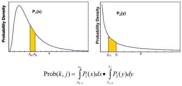
As next step the user can select the kind of statistical evaluation. Two methods are available. The first is the well known Monte-Carlo simulation. For this method a combination of the distributed parameters will be selected by chance and the crack propagation for a given time period is calculated. If the investigated pipe fails during that calculation the time of failure and the failure mode are saved. This will be repeated with a user prescribed number of trials depending on the expected failure probability. The second option is a stratified integration method based on a variance reduction technique. For this method the user can select two out of all distributed parameters (usually the crack depth and the crack length to depth aspect ratio) to be integrated bit by bit. The whole range of both selected parameters is divided into user defined cell numbers. A set of the other distributed parameters is selected by chance. The crack propagation for a given time period is calculated for each cell combination together with this set. If the pipe fails during that calculation the time of failure, the probability of the actual combination and the failure mode are saved. The probability of the actually considered cell combination (k,j) is the product of the corresponding single cell probability (see figure 1). This will be repeated with a user prescribed number of trials (100 are recommended) which then allows an evaluation of the failure probability together with an uncertainty range.
x xk xk-1 P ro b ab ility D en
sity P1(x)
x xk xk-1 P ro b ab ility D en sity x xk xk-1 P ro b ab ility D en
sity P1(x)
y yi yi-1 P ro b ab ility D en
sity P2(y)
y yi yi-1 P ro b ab ility D en sity y yi yi-1 P ro b ab ility D en
sity P2(y)
∫
∫
− −•
=
j j k k y y x xdy
y
P
dx
x
P
j
k
1 1)
(
)
(
)
,
(
Prob
1 2Fig. 1: Probability of cell combination for stratification method.
The residual stresses can be set to be active or not. If they are active the user has to input the values of the residual stresses along the wall thickness. Similar to the stress load set the stress level can be specified at eight user defined wall thickness positions and at the inner and outer surface point.
The user can choose if he wants to consider in service inspections (ISI) in the calculation. If this choice is active he is requested to input a probability of detection (POD) curve of non destructive examination techniques. The user can determine the POD curve by specifying ten crack depth values and their corresponding detection probabilities in percent together with the time inspection interval. Internally this data are used to identify if a crack is detected during an inspection or not. An inspection changes the probability of the crack by multiplying it with the value of not detecting the crack which is one minus the POD curve value for the actual crack depth.
Calculation procedure
Before running the problem the user is requested to give some more run time data. These are the number of years that should be calculated, the number of intervals for the integration parameters if the stratified integration option was selected, the number of trials that should be investigated and the seed value of the random generator. Additionally the user has two options regarding the calculation of the limit load. The first one is an approach of Kiefner [4] and the second one is an approach for axial and circumferential semi elliptical inner surface cracks in pipes described in the Ductile Fracture Handbook (DFH) [5].
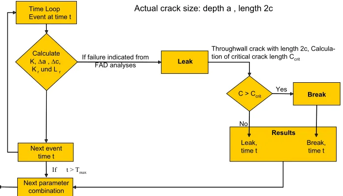
Let P1, P2….PA be the distributed parameters of our problem, N the number of trials and tmax the calculation time. If the Monte-Carlo simulation is active a parameter set of P1, P2….PA is selected by chance. The actual time t starts at 0 and the next event time t is calculated by the given frequencies of the load sets or the ISI interval. At time t the stress intensity factor K at the deepest and at the inner surface crack front position are estimated together with the resulting crack growth ∆a and ∆c. For this new crack size a failure assessment according to the SINTAB Level 1B procedure [6] tests if the limiting conditions are exceeded. If so, a leak occurs and the semi elliptical crack is assumed to be a through wall crack of actual crack length size. If the crack length exceeds the critical crack length ccrit a break appears. If the crack is smaller than the critical length only a leak appears. In either case the failure time and mode is saved and the calculation starts with a new parameter set P1, P2….PA. If the limiting FAD (Failure Assessment Diagram) conditions are not exceeded the next event time t is calculated. This is done until t is larger than tmax or the crack failed. Figure 2 illustrates schematically the procedure. The whole procedure is repeated N times. It is recommended to use a trial number which at least results in 10 to 100 failures.
If the stratified integration option is selected with stratified parameters P1 and P2 a parameter set of P3….PA is selected by chance. A loop over all combinations of P1 and P2 (interval number of P1 * interval number of P2) starts and the time calculation identical to the Monte-Carlo option is performed for every combination. If a combination leads to failure of the pipe, time t, failure mode (leak or break) and combination probability is saved. After that a new parameter set P3….PA is selected until the number of trials N is reached. For an uncertainty analysis it is recommended to use N=100 and interval numbers of 10-100 depending on the distribution functions of P1 and P2. We have made a good experience with a crack depth interval number of 20 and a crack length interval number of 10. With this method 10*20*100=20000 combinations are calculated to reach the same confidence in the results as in a Monte-Carlo simulation independently of the failure probability. So this method is much faster than a Monte-Carlo simulation if the leak or break probability is below 1.0*E-3. Additionally an uncertainty analysis of the leak and break probability distribution can be performed.
Time Loop Event at time t
If failure indicated from FAD analyses Calculate
K, ∆a , ∆c, Krund L r
Leak
Break
Actual crack size: depth a , length 2c
Next event time t
If t > Tmax
Next parameter combination
Throughwall crack with length 2c, Calcula-tion of critical crack length Ccrit
Yes
No C > Ccrit
Results Leak,
time t
Break, time t
Output and results
The regular output file (xxx.out) contains the information about all given input parameters including the run time variables. Then for all combinations that fail the actual parameter values, failure time, failure mode, crack depth, crack length, stress intensity factors for the maximum and minimum load at deepest and surface point and the combination probability are listed in the output file. In a second output file (xxx.plt) the accumulated failure probability is listed as a function of time. If the stratified integration method was selected processed 5%, 50% and 95% failure probability curves as a function of time are listed too. The 50% curve represents the expected failure probability that is equivalent with the results of a Monte-Carlo run depending strongly on the mean values of the distribution functions of the input parameters. The 5% and 95% curves depend strongly on the shape of the distribution functions of the input parameters and show the uncertainty range of the 50% curve. It represents the area of the failure probability with approximately 90% statistical confidence. To gain this uncertainty area each accumulated failure time history of the 100 runs is fitted by a Weibull curve and then the 5th highest and lowest value of all curves is listed for each time.
INFLUENCE OF DIFFERENT OPTIONS ON THE RESULTING LEAK PROBABILITY
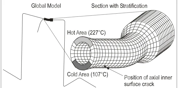
The influence on the failure probability by changing the options for the stress intensity factor and limit load calculation will be exemplary shown on a part of an austenitic German PWR piping system with postulated axial inner surface crack size distribution subjected to a combined load of 15.5 MPa internal pressure and a thermal stratification. It was assumed that the thermal stratification conditions appear every 320 minutes (1640 cycles/year) with a high temperature area of 227°C at the top of the pipe (10-2 o’clock) and a low temperature area of 107°C at the bottom of the pipe (4-8 o’clock). A finite element model of the piping system was generated. It consists of 20 node brick elements in the part where the thermal stratification occurs and of pipe elements elsewhere. Figure 3 illustrates the model. The pipe wall thickness at the assumed crack position section was 6.3 mm and the outer diameter 60.3 mm. Stress intensity factors were calculated via J-integral values from included crack models with 2, 3 and 4 mm crack depth and with half crack length to depth aspect ratios (c/a) of 2, 3 and 4. From these results the coefficients A1-A16 of formula (2) are gained as input for the user defined stress intensity factor calculation in PROST. Additionally one calculation without any crack was done to get the crack opening stress along the wall thickness at the crack location. Figure 4 shows the crack opening stress at this position at that time where the highest loading occur.
Fig. 3: Finite element model of the piping system
Probabilistic calculations of this problem were performed with PROST. The input data set of the parameter values are given in table 1. The crack depth distribution includes large deep cracks, 50% of the cracks are deeper than half of the wall thickness. It was artificially set to this high values, because we only wanted to do parametric studies with some of the PROST options and a high probability of large cracks reduces the calculation time with the Monte-Carlo option significantly.
Parameter Type of
function
Mean value (median)
Standard Deviation
95% Quantile Minimum Maximum
Inner radius [mm] Normal 23.85 0.25 - 23.5 24.2
Wall thickness [mm] Normal 6.3 0.4 - 5.5 7.1
Crack depth [mm] Log-normal 3.15 - 5.0 0.0 5.3
c/a Exponential 2 - - 1 20
Young’s modulus [GPa] - 185 - - -
-Fracture toughness [MPa m1/2] Normal 266 20 - -
-Flow stress [MPa] Normal 310 32 - 263 449
Yield stress [MPa] Normal 178 25 - 130 240
Ultimate strength [MPa] Normal 442 32 - 390 605
Growth law constant C
[mm/Cycle/ (MPa m1/2)m] Log-normal 5.06E-10 - 1.26E-8 2.8E-13 9.19E-7
Growth law exponent m - 3.93 - - -
-Threshold ∆K [MPa m1/2] - 3.0 - - -
-Table 1: Input data set of axial crack example
Influence of stress intensity factor calculation
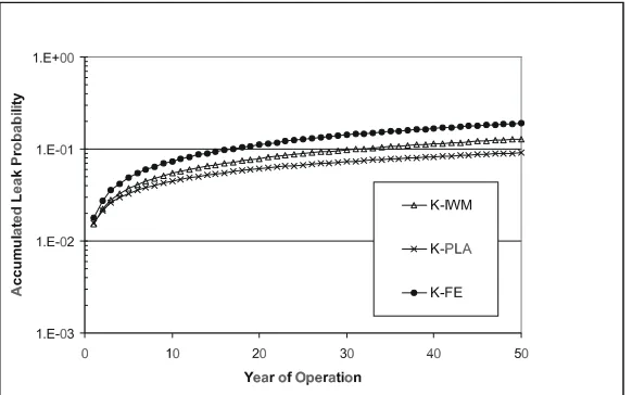
In a first stage we studied the influence of the stress intensity factor calculation on the leak probability of the pipe. For simplification we set all parameters except the crack depth and the c/a ratio to mean values. All calculations have been done with the stratified integration option and 20x10 intervals for the crack depth and c/a ratio respectively and a limit load approach described in the DFH [5]. Figure 5 illustrates the resulting accumulated leak probabilities as a function of operation time for the three different stress intensity factor calculation options. The highest leak probabilities appear with the stress intensity factors based on the finite element calculation (K-FE) and reach a value of about 0.2 after 50 years. The lowest values appear with the weight function method of an equivalent loaded plate (K-PLA). They reach a value of nearly 0.1 after 50 years, a factor of 2 lower than the K-FE values. In between are the results with the influence function procedure described in [2] (K-IWM). In the first years all results agree very well, because the leak probability in this area is controlled by the limit load approach only, which is the same in all cases. A more detailed investigation of the K-values shows that the values of the IWM approach agree very well with the FE-values in the crack size range investigated with the FE-model, which is 2-4 mm crack depth and c/a ratio of 2-4. Outside of this range the extrapolated FE-values exceed the IWM-values which results in a higher crack growth and a larger leak probability, whereas the equivalent loaded plate K-values are consequently lower for all crack sizes compared to the other methods.
Influence of limit load approach
In a second stage we investigated the influence of the limit load approach on the leak probability of the pipe. We have done these calculations with the same input data set as used in the K-variation case. Figure 6 shows the resulting leak probabilities with a limit load approach of the ductile fracture handbook (DFH) [5] and an approach by Kiefner [4]. In both cases the K-values are calculated with the IWM procedure [2]. Changing the limit load means changing the maximum allowable crack size that leads to failure. The DFH [5] approach is more conservative than the Kiefner approach and results in significant higher leak probabilities especially in the first years. They differ in one order of magnitude at the beginning and in a factor of 1.7 after 50 years.
Fig. 6: Comparison of leak probability time history for different limit load calculations
As a result we can conclude that the influence of the used limit load approach on the leak probability is of the same order as using different K-calculation techniques for a large number of cycles, but very significant for a low number of cycles. The higher the number of cycles the more important is the used stress intensity factor calculation, whereas the lower the number of cycles the more important is the used net section collapse criterion.
Influence of statistical evaluation
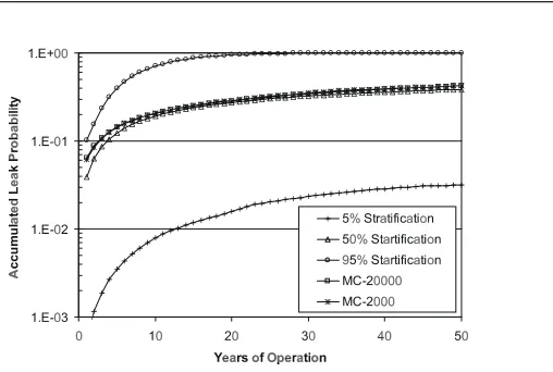
To investigate the difference of the two available statistical methods we performed calculations with all parameters distributed as given in table 1. We have selected the IWM stress intensity factor calculation and the DFH limit load approach. For the stratified integration method we used the 20x10 intervals for the crack depth and the c/a ratio as before, but now we have calculated 100 sets of the other distributed parameters selected by chance. In all we calculated 10x20x100=20000 combinations. For the Monte-Carlo (MC) option we have performed a calculation with 20000 combinations too. Figure 7 shows the resulting leak probabilities.
Fig. 7: Comparison of leak probability time history for different statistical evaluations
statistical confidence area was evaluated from the calculation with the stratified integration option shown by the 5% and 95% curve.
COMPARISON BETWEEN PROST AND PRAISE RESULTS
The original PRAISE 3.10 was designed for circumferential cracks only. This code was supplemented by GRS with an option for calculating axial cracks without changing the calculation routine for circumferential cracks. Additionally the statistical evaluation has been changed to the stratified integration method described above, but as shown in figure 7 the results of the 50% curve are equivalent with Monte-Carlo results. To compare PROST and PRAISE results we have calculated an example with a postulated circumferential crack distribution.
We considered a fictitious case of a weld in an austenitic pipe with an inner radius of 33.4 mm and 11.1 mm wall thickness subjected to a cyclic loading condition. The crack opening stress reach at the maximum a constant level of 94 MPa and at the minimum a constant level of 23 MPa which corresponds to an internal pressure of 15.4 MPa. The loading appears 1000 times a year. For simplification all parameters except the crack depth are set to the mean values given in table 2.
Parameter Mean value Parameter Mean value
a/c 3 Ultimate strength [MPa] 450
Young’s modulus [GPa] 180 Growth law constant C [mm/Cycle] 5.06E-10
Fracture toughness [MPa m1/2] 266 Growth law exponent m 3.93
Flow stress [MPa] 300 Threshold ∆K [MPa m1/2] 0.0
Yield stress [MPa] 150
Table 2: Input data set of circumferential crack example
For the pre existing crack depth distribution in the weld we have used a Log-normal function with a much lower probability for large cracks compared to the first example. The mean value was 1.8 mm and the 95% quantile was 4 mm. Only 1% of the cracks is deeper than half of the wall thickness and only cracks larger than 8.8 mm contributes to the leak probability. These largest cracks have a probability density of about 10-7. The used distribution function is similar to results calculated with the RR-PRODIGAL program [7].
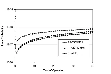
The PROST calculations of this problem have been performed with the IWM stress intensity factor procedure and both limit load options DFH and Kiefner. In the calculation with the stratified integration method, the crack depth was separated into 100 intervals. In the Monte-Carlo calculation 20000/100000 crack depths selected by chance have been investigated. In the PRAISE calculation a separation into 100 crack depth intervals has been used too. The stress intensity factor procedure and the net section collapse criterion are still the original ones of PRAISE. They can not be changed by a user input option. Figure 9 shows a comparison of the resulting leak probabilities. They are in the order of 10E-7 and the PROST and PRAISE results agree nearly perfectly if the IWM K-value option and a limit load by Kiefner is used in PROST. Again it is seen that the DFH limit load option is more conservative and leads to higher failure probabilities. It can be concluded that the different failure determination methods of the two codes have no significant influence on the resulting leak probability.
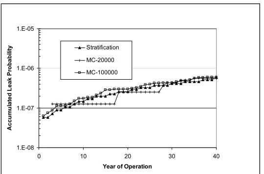
Figure 10 illustrate a comparison of the resulting leak probabilities of the above problem by using the stratified integration method and the Monte-Carlo method respectively. With the stratified integration option the program needs 35 seconds to calculate the probability curve resulting from the 100 crack depths. A Monte-Carlo run with 20.000 trials lasts 2 hours and 15 minutes and does not meet the leak probability very well. A 100.000 trial run needs 11 hours to reach nearly the same values as the stratified integration method does.
1.E-08 1.E-07 1.E-06 1.E-05
0 10 20 30 40
Year of Operation
Leak
P
robabi
lit
y
PROST-DFH PROST-Kiefner PRAISE
1.E-08 1.E-07 1.E-06 1.E-05
0 10 20 30 40
Year of Operation
A
c
cu
m
u
la
te
d
L
eak
P
ro
b
a
b
ili
ty Stratification MC-20000 MC-100000
Fig. 10: Leak probability of stratified integration and Monte-Carlo option calculated with PROST
CONCLUSIONS
With the present version of the PROST development parametric studies were performed to investigate e.g. the influence of different stress intensity factor calculation methods and net section collapse criteria on the resulting leak probabilities of fatigue problems. The higher the number of cycles the more important are differences in the stress intensity factor calculation, whereas the lower the number of cycles the more important are the differences in the net section collapse criteria. The presented statistical stratification method can save a lot of calculation time compared to a Monte-Carlo method if the expected failure probabilities are low. Furthermore a statistical confidence area can be evaluated with this method. A comparison of resulting leak probabilities calculated with PROST and with the public available US code PRAISE shows that good agreement could be achieved. Further development is in progress especially to perform investigations on stress corrosion cracking as a damage mechanism.
REFERENCES
1. Harris, D.O., Dedhia, D., Theoretical and User’s Manual for pc-PRAISE, NUREG/CR-5864, UCRL-ID-109798, 1992.
2. Busch, M., Petersilge, M., Varfolomeyev, I., Polynomial Influence Functions for Surface Cracks in Pressure Vessel Components, Fraunhofer Institut für Werkstoffmechanik (IWM)-Report Z 11/95, 1995
3. Shen, G., Plumtree, A., Glinka, G., Weight Function for the Surface Point of Semielliptical-Surface Crack in a Finite Thickness Plate, Engineering Fracture Mechanics, Vol. 40, No.1, pp.167-176, 1991
4. Kiefner, J.F., et al., Failure Stress Levels of Flaws in Pressurized Cylinders, ASTM STP 536, pp.461-481, 1973 5. Zahoor, A., Ductile Fracture Handbook, EPRI NP-6301, Vol.3, 1991
6. Zerbst, U., Wiesner, C., Kocak, M., Hodulak, L., SINTAP: Entwurf einer vereinheitlichten europäischen Fehlerbewertungsprozedur- eine Einführung, GKSS 99/E/65, 1999