Real Time Predictive Speed Analysis for High Speed Rail Collision Test

(1)

University of Windsor University of Windsor

Scholarship at UWindsor

Electronic Theses and Dissertations Theses, Dissertations, and Major Papers

10-19-2015

Real Time Predictive Speed Analysis for High Speed Rail Collision

Test

Xian Jian Jiang

University of Windsor

Follow this and additional works at: https://scholar.uwindsor.ca/etd

Recommended Citation Recommended Citation

Jiang, Xian Jian, "Real Time Predictive Speed Analysis for High Speed Rail Collision Test" (2015). Electronic Theses and Dissertations. 5441.

https://scholar.uwindsor.ca/etd/5441

This online database contains the full-text of PhD dissertations and Masters’ theses of University of Windsor students from 1954 forward. These documents are made available for personal study and research purposes only, in accordance with the Canadian Copyright Act and the Creative Commons license—CC BY-NC-ND (Attribution, Non-Commercial, No Derivative Works). Under this license, works must always be attributed to the copyright holder (original author), cannot be used for any commercial purposes, and may not be altered. Any other use would require the permission of the copyright holder. Students may inquire about withdrawing their dissertation and/or thesis from this database. For additional inquiries, please contact the repository administrator via email

(2)

Real Time Predictive Speed Analysis for High

Speed Rail Collision Test

By

Xian Jian Jiang

A Thesis Submitted to the Faculty of Graduate Studies through Computer Science in Partial Fulfillment of the Requirements for the Degree of Master of Science at

the University of Windsor

Windsor, Ontario, Canada

2015

(3)

Real Time Predictive Speed Analysis for High Speed Rail Collision Test

by

Xian Jian Jiang

APPROVED BY:

_______________________________________________________

Dr. Guoqing Zhang Department of Mechanical, Automotive and Materials Engineering

_______________________________________________________

Dr. Arunita Jaekel School of Computer Science

_______________________________________________________

Dr. Dan Wu, Advisor School of Computer Science

(4)

Author’s Declaration of Originality

I hereby certify that I am the sole author of this thesis and that no part of this

thesis has been published or submitted for publication.

I certify that, to the best of my knowledge, my thesis does not infringe upon

anyone’s copyright nor violate any proprietary rights and that any ideas, techniques,

quotations, or any other material from the work of other people included in my thesis,

published or otherwise, are fully acknowledged in accordance with the standard

referencing practices. Furthermore, to the extent that I have included copyrighted

material that surpasses the bounds of fair dealing within the meaning of the Canada

Copyright Act, I certify that I have obtained a written permission from the copyright

owner(s) to include such material(s) in my thesis and have included copies of such

copyright clearances to my appendix.

I declare that this is a true copy of my thesis, including any final revisions, as

approved by my thesis committee and the Graduate Studies office, and that this

thesis has not been submitted for a higher degree to any other University or

(5)

Abstract

In a real train collision test, a train locomotive needs to be propelled on a straight,

guided path, to a particular speed, at which time the train locomotive is released to

coast down towards a barrier where it is required to crash at a desired speed. The

current control of the release speed and location is based on theoretical data and

previous experience which leads to less accuracy in the actual crash speed. In this

research work, the goal is to make improvements in a typical real train collision test

that will help obtain a more accurate crash speed and release location by controlling

the force release precisely. The contribution of this research work is to implement a

solution to simulate the behavior of the propulsion system, and trigger an algorithm

to calculate the required release speed and location more accurately and quickly.

(6)

Dedication

This thesis is dedicated to my wife who has supported me all the way since the

beginning of my studies.

(7)

Acknowledgements

First of all, I would like to express my deep and sincere gratitude to my

supervisor, Dr. Dan Wu, for his invaluable guidance and advices, for his enthusiastic

encouragement and his great patience to me. Without his help, the work presented

here would not have been possible.

A very special thanks goes out to Mr. Roland Vander Straeten of Anemoi

Technologies Inc. Mr. Roland Vander Straeten is the one specialist who truly made

a difference in my life. It was under his tutelage that I developed the current

application software and became interested in the state-of-the-art test facilities. He

provided me with direction, technical support and became more of a mentor and

friend, than an employer.

I would also like to thank my external reader, Dr. Guoqing Zhang, and my

internal reader, Dr. Arunita Jaekel, for spending their precious time to review this

thesis and putting down their comments, suggestions on the thesis work.

Finally, I am very grateful for experts of Anemoi Technologies Inc., Jessica

Zheng, Mike Doiron, Slawek Ciurzynski and Bruce Hu. During these two years’

study, they gave me great and solid support whenever I met any kind of problems.

They always share their valuable knowledge and experiences with me. This is the

(8)

LIST OF TABLES

3.1 Leading Time Calculation .………..………...51

4.1 Run with Different Set of Data...………...61

4.2 Run with Different Values of Crash Speed………....……….62

4.3 Run with Different Values of Barrier Location………...……...63

4.4 𝑅²for Speed of 60kph..………...…...………...63

4.5 𝑅²for Speed of 80kph………..……….………...63

4.6 𝑅²for Speed of 120kph………..….………..…………...64

4.7 𝑅²for Speed of 150kph..………...64

4.8 𝑅²for Different Error Ratios………...64

(11)

LIST OF FIGURES

1.1 Deadly Collision ……..……….4

2.1 Data Distribution of Lean Body Mass and Muscle Strength………...11

2.2 Simple Linear Regression - Straight Line….……….……… 12

2.3 Different Fitted Lines for A Set of Data……..……….……… 13

2.4 Vertical Distance vs Perpendicular Distance………14

2.5 Propulsion–Release Force–Coast Down ……….………21

2.6 Train and Track…...……….………22

2.7 Building Housing the Rigid Wall……….…………22

2.8 Rigid Wall………..……….…………22

2.9 Sample Data 1……….………25

2.10 Sample Data 2……….………26

3.1 Small Intervals of Propulsion Curve………….………31

3.2 Start and End Points for Simulations………...………33

3.3 System Architecture………...………35

3.4 Software Structure……….…….………36

3.5 Intersection Point………...…….………38

3.6 The Format of Simulated Data Stream…….………39

3.7 Main Process of 𝑅𝑇𝑃𝑆𝐴………41

3.8 End Point for Data Collection ……….………43

3.9 Program Logic of Coefficients Calculation………45

3.10 Time-Equal Intervals for Coast-Down Simulation………47

3.11 Coast-Down Curves ……….………48

3.12 Program Logic of Coast-down Simulation ……….………49

3.13 Start Point for Propulsion Simulation ……….………50

3.14 Program Logic of Propulsion Simulation …………...………53

3.15 Program Logic of Control and Release Processing……..………55

4.1 Screen Shot of Demonstration Program…………..………58

(12)

4.3 Output Screen of the Standalone Version….……..………60

4.4 Screen Shot of Console - Running Time …………..………60

4.5 Maximum Propulsion Force = 60,000………..………66

4.6 Maximum Propulsion Force = 70,000………..………66

(13)

Chapter 1 Introduction

1.1 Introduction of High Speed Rail

The global high speed rail (HSR) network is one of the great feats of modern

engineering, and proves to be one of the best forms of transportation ever

invented. The global HSR network is rapidly expanding across continents world

wide - delivering fast, efficient mobility to numerous nations every day [35].

HSR is currently in operation in more than twenty countries (including the UK,

France, Germany, Belgium, Spain, Italy, Japan, China, Korea, and Taiwan)

[34]. HSR is under construction in more than ten countries (including China,

Spain, Saudi Arabia, France, and Italy). In the meantime, it is in development in

another fourteen countries (including Turkey, Qatar, Morocco, Russia, Poland,

Portugal, South Africa, India, Argentina, and Brazil). In Japan, HSR has been in

operation for fifty years carrying more than nine billion passengers without a single

fatality [31].

HSR delivers many layers of economic benefits. It is one of the solutions to

rising gas prices. HSR delivers fast, efficient transportation so riders can save time,

energy, and money. It is reliable and operates in almost all weather conditions

[12]. HSR is not subject to congestion, so it operates on schedule every day without

delay - especially during rush hour and peak travel times.

HSR stimulates the revitalization of cities by encouraging high density,

mixed-use real estate development around the stations [35]. It also fosters economic

(14)

integrated regions that can then function as a single stronger economy. HSR can

generate more job opportunities to labor markets and offers workers a wider network

of employers to choose from. It also encourages and enables the development of

technology clusters with fast and easy access between locations. In the meantime, it

also expands tourism markets while increasing tourists spending.

1.2 Brief History of HSR

High-speed trains were first introduced in the early 19th_{century when British}

engineers developed the steam railroad locomotives [1]. These locomotives were the

beginning of a long era in which various technologies were pursued in order to

achieve higher speeds coupled with operating and fuel efficiencies. Steam

propulsion gave maximum speeds of about 160kph (100mph) in the early 20th

century. Test speeds of 209kph (130mph) were attained by using diesel-electric and

electric propulsion in the 1930s and 1940s. This change in technology provided

slightly improved performance and fuel efficiency, but it was not until the 1960s that

breakthroughs in suspension, train–track dynamics, and other factors permitted an

increase in train speeds.

On November 1st_{, 1965, the Japanese introduced, as part of the regular train}

schedule, a standard-gauge railway service that reached the maximum speed of

209kph (130mph) [31]. The average speed of the train was 166kph (103mph). The

Pennsylvania railroad developed the “metro-liners” by placing traction motors on

each axle [33]. That train achieved the maximum speed of 251kph (156mph) in

Princeton, New Jersey, in May 1967. Only a decade ago, “metro-linerlike” coaches

pulled by AEM-7(Asea Electro Motive 7000hp) locomotives operating at speeds of

up to 201kph (125 mph) in service were the only relatively high-speed rail systems

in the United States [35]. At present, high-speed rail trains regularly operate in Japan,

France, Germany, and other countries worldwide in service, at speeds between 240

(15)

(bullet train) between Osaka and Tokyo for more than thirty years [31].

The French initiated high-speed service between Paris and Lyon with the TGV

(Train à Grande Vitesse - French high speed train) in 1981 [32]. The latest French

TGV trains operate in service on several lines (about 25% of the lines are dedicated

to their use) connecting Paris with Brussels, London (under the British Channel,

called the Eurostar), and cities of the Atlantic and Mediterranean coasts. The TGV

achieves peak speeds of 320kph (200mph) and has been tested at a sustained speed

of 515kph (330mph). Similarly, the Germans operate their own ICE

(Inter-City-Express Train) all over the country (using mainly non-dedicated lines).

HSR in China may refer to any commercial train service in China with an

average speed of 200kph (124mph) or higher [29]. By that measure, China has the

world's longest HSR network with over 11,028 km (6,852 mi) of track in service as

of December 2013, including the world's longest line, the 2,298 km (1,428 mi)

Beijing–Guangzhou High-Speed Railway.

Since high-speed rail service in China was introduced on April 18th_{, 2007, daily}

ridership has grown from 237,000 in 2007 to 1.33 million in 2012, making the

Chinese high-speed rail network the most heavily used in the world [34]. China's

high-speed rail network consists of upgraded conventional railways, newly built

high-speed passenger designated lines (PDLs), and the world's first high-speed

commercial magnetic levitation (maglev) line. Nearly all high-speed rail lines

and rolling stock are owned and operated by the China Railway Corporation, the

national railway operator formerly known as the Railway Ministry. The Shanghai

Maglev Train is owned and operated by Shanghai's city government [29].

China's early high-speed trains were imported or built under technology transfer

(16)

components and built indigenous trains that can reach operational speeds of up to

380kph (240mph).

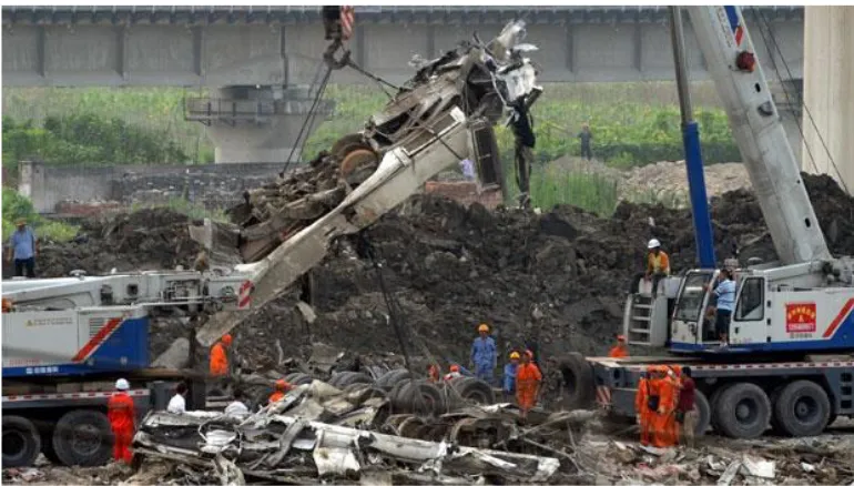
1.3 Safety Issues and Technology

As the speed of trains becomes faster and faster, the severity of accidents can

be disastrous. In the city of Wenzhou, China on July 24th_{, 2011, a deadly collision}

happened and over forty people were killed in this accident. It was caused when one

train, struck by lightning, lost power and a second train crashed into its back [11].

Figure 1.1 shows the rescue effort.

Figure 1.1 Deadly Collision. Source: CBC NEWS

Another accident happened in Bulgaria on July 12th_{, 2014. A long distance}

passenger train derailed at Kaloyanovets station, killing the driver and injuring

fourteen others. The train passed through turnouts set to diverging track at 104kph.

A large part of the research regarding high speed ground transportation systems

has focused on safety issues [36]. Many of these issues deal with crash tests and car

(17)

While train collisions are extremely rare occurrences, when one happens, heavy

casualties are almost unavoidable. For this reason, many European countries and the

USA have developed design methods to minimize damage in the event of a train

collision [37]. Moreover, in an effort to improve train crashworthiness, these

countries have developed safety guidelines for passenger trains. One aspect of such

efforts is to apply design to the car and make it crushable, thereby absorbing energy

[38]. Those techniques include improved crashworthiness cab car and locomotive

structural designs [5, 6], improved crashworthiness coach car structural designs [7],

and a variety of interior occupant protection strategies [8]. Since the setup of real

train collision test facility requires massive amounts of time and expense, such a

technique was rarely used before. Therefore, simulation methods are particularly

important in the train collision testing field. So far, crashworthiness has been

assessed using four modeling techniques. The first is to sequentially analyze and

evaluate the partial structure of a train by using a 3D finite element modeling

techniques [1]. The second is to analyze the crushing characteristics of the entire

train by applying the crushing characteristics obtained from the first technique to a

1D train model [2]. The third is to use a 2D modeling technique to estimate

overriding [3]. The fourth is a technique to predict the behavior of an entire train by

using a 3D multi-body dynamics model [10]. Although these methods have been

efficiently applied in computer system without much difficulty, they have many

restrictions in terms of their ability to predict the nonlinear collision behavior that

occur in an actual collision [39]. In other words, the aforementioned evaluation

methods all have the shortcoming that they cannot consider interactions sequentially

occurring among each component, suspension, bogie and the body [40].

As a matter of fact, the most ideal technique providing the highest reliability in

predicting collision behavior is to use a real train collision [41]. Another main

purpose of doing the real train collision test is to validate the simulation code because

it is much cheaper to run the computer code than crashing an actual train. In the

(18)

of this thesis are highlighted, and the structure of the remaining chapters are outlined.

1.4 Motivation

The most ideal technique providing the highest reliability in predicting collision

behavior is to use a real train collision, but this does requires massive amounts of

time and expense [41]. In the real train collision test, a train locomotive needs to be

propelled on a straight, guided path, to a particular speed, at which time the train

locomotive is released to coast down to a crash barrier where it is required to crash

at a desired speed. That propulsion could be in the form of a cable pulling the train

inside a laboratory setting or another locomotive pushing the test object along a long

train track. The current control of the release speed and the release location is based

on theoretical data and previous experience which leads to less accuracy in

controlling the actual crash speed. The resistance forces, including inertia, friction

and aerodynamic resistance forces, are playing important roles and significantly

influence the behavior of both propulsion and coast-down movement. And due to

the lack of a mechanism to collect the real-time data to calculate the resistance force

along the test, the current release speed and location is only roughly estimated.

Inaccuracy of crash speed means the waste of great deal of time and money. The

motivation in this thesis is to design and implement a solution to simulate the

performance data from the propulsion phase, and trigger an algorithm to calculate

the release speed and location more accurately and quickly. The critical works in

this solution are to implement a proper mathematical model to describe and analyze

the behavior of resistance force, calculate the regression coefficients quickly,

simulate the coast-down process and find the release speed and location precisely.

1.5 Contributions

This thesis is concerned with the problem of mathematical models to analyze

(19)

behavior. The contributions of this thesis are as follows.

The primary contribution of this thesis is that a regression analysis data model

is applied to analyze the data set obtained from industry experts that is used to

calculate and estimate the real time performance of the testing vehicle, such as forces,

acceleration, [pulling cable] motor torque, speed and location. In a real testing

environment, such data will be collected in a real time basis through an array of

sensors. After the calculation based on the provided data set, a new data set is

obtained describing the relationship between resistance force and speed. The least

squares method is then applied to calculate and determine the regression coefficients

which in turn leads to a best fit function of resistance to describe the behavior of the

new obtained data set. This resistance function will be used later on to predict the

performance of resistance force for coast-down movement as well as for the

propulsion behavior.

The second important contribution is that a practical approach is designed and

implemented to simulate the coast-down behavior. The coast-down movement starts

at the release location where the propulsion force is released and it ends at the

position of collision between the test vehicle and the barrier. There are several

difficulties in such a simulation. For example, the location and speed of the start

position of coast-down are unknown and the whole coast-down movement is a

varying acceleration motion. In order to solve this problem, a reverse analysis is

designed and provided in this research. The coast-down simulation is done by

calculating the speed and location at each time stamp starting from the end position

of the coast-down movement instead of the start position, because the speed and

location for the end position, which means the crash speed and location of barrier,

are predefined and known.

(20)

of the design and development are presented, such as system architecture, software

structure, design principles, program logic and flows chart. This software application

is part of the overall control system (Facility Control System) in a real test facility.

The data-feed interface in this application can be easily modified to adapt to the real

interface to measuring sensors. This software can also be customized as a standalone

tool to let the users be able to change and manipulate different parameters to simulate

different scenarios.

1.6 Guide to the Thesis

This thesis is organized as follows.

Chapter 2: Background Knowledge. This chapter provides an introduction to the subject that the proposed method builds upon. The theory of regression analysis will

be reviewed at first. Multiple linear regression and least squares method are

specifically emphasized, since they are the core and foundation of the proposed

approach. After the introduction of regression analysis, the idea of real train collision

test and some major concepts will be explained.

Chapter 3: Proposed Solution - 𝑹𝑻𝑷𝑺𝑨. The proposed method is presented and explained in this chapter which covers the major contribution of this thesis to fulfill

this research work. The software developed is called 𝑅𝑇𝑃𝑆𝐴 (Real Time Predictive

Speed Analysis). The definition of the problem is described in the beginning of this chapter, followed by objective and design principles of the proposed approach. Then,

system architecture and software modules will be introduced in detail. After reading

this chapter, readers will be able to understand the advantages of the proposed

method and the implementation details in this research work.

(21)

presented, together with explanation and analysis of the result tables. This leads to

the conclusion in following chapter.

(22)

Chapter 2 Background Knowledge

This chapter provides the background knowledge on which the proposed

method is based. The theory of regression analysis will be reviewed which includes

simple linear regression, multiple linear regression, the calculation of regression

coefficients and the correlation coefficients. After that, test phases, typical setup in

a real train collision test, an in-depth knowledge of the vehicle motion and sample

data sheet will be introduced.

2.1 Regression Analysis

Regression analysis is a statistical technique for the investigation of

re-lationships between variables [13]. Usually, the investigator seeks to ascertain the

causal eﬀect of one variable upon another—the eﬀect of a price increase upon

demand, for example, or the eﬀect of changes in the money supply upon the inflation

rate [19]. To explore such issues, the investigator assembles data on the underlying

variables of interest and employs regression to estimate the quantitative eﬀect of the

causal variables upon the variable that they influence. The investigator also typically

assesses the “statistical significance” (correlation coefficient) of the estimated

relationships, that is, the degree of confidence that the true relationship is close to

the estimated relationship [20].

The goal of regression analysis is to determine the values of parameters for a

function that cause the function to best fit a set of data observations provided.

(23)

2.1.1 Simple Linear Regression

In its simplest form, linear regression shows the relationship between one

independent variable 𝑋 and a dependent variable 𝑌, as in the formula below:

𝑌 = 𝑎0+ 𝑎1𝑋 + 𝑢 (2.1)

The magnitude and direction of that relationship are given by the slope parameter𝑎₁,

and the status of the dependent variable 𝑌 when the independent variable 𝑋 is 0 is

given by the intercept parameter 𝑎₀. An error term 𝑢 captures the amount of

variation not predicted by the slope and intercept terms [14].

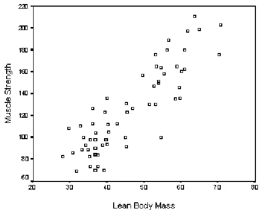
An example of simple linear regression is the relationship between muscle

strength against lean body mass. Figure 2.1 shows a data distribution about them.

Figure 2.1 Data Distribution of Lean Body Mass (kg) and Muscle Strength

(kg/cm²). Source: [46]

The 𝑋-axis in Figure 2.1 represents lean body mass while the 𝑌-axis represents

muscle strength. Each small square is a pair of data of (𝑥, 𝑦). By observing Figure

(24)

relationship isn't perfect because it's easy to find two people where the one with more

lean body mass is the weaker, but in general strength and lean body mass tend to go

up and down together. When two variables are displayed in a scatterplot and one can

be thought of as a response to the other (here, lean body mass produces strength),

standard practice is to place the response on the vertical (or 𝑌) axis. The names of

the variables on 𝑋 and 𝑌 axes vary according to the field of application. Some of

the common usages are as follows.

X-axis Y-axis

independent dependent predictor predicted

carrier response

input output

The association between lean body mass 𝑋 and muscle strength 𝑌 looks like

it could be described by a straight line shown in Figure 2.2.

Figure 2.2 Simple Linear Regression - Straight Line. Source: [46]

The data (each small square) are pairs of independent and dependent variable

values {( 𝑥_𝑖, 𝑦_𝑖): 𝑖 = 1, … , 𝑛}. The fitted function could be written as

ŷ = 𝑏₀+ 𝑏₁𝑥 (2.2)

(25)

and 𝑏1 are regression coefficients. The residuals are the differences between the

observed and the predicted values {( 𝑦_𝑖− ŷ_i): 𝑖 = 1, … , 𝑛}.

There are two primary reasons for fitting a regression function to a set of data.

The first is to describe the data and the second is to predict the dependent variable

value from the independent variable value. The method of calculation for the fitted

regression function will be introduced in Section 2.1.4 and the rationale behind the

way the regression line is calculated is best seen from the point-of-view of prediction

[21]. A line gives a good fit to a set of data if the points are close to it. Figure 2.3

shows that there could be many different lines to fit the data set. Where the points

are not tightly grouped about any lines, a line gives a good fit if the points are closer

to it than to any other lines. For predictive purposes, this means that the predicted

values obtained by using the line should be close to the values that were actually

observed, that is, the residuals should be small. Therefore, when assessing the fit of

a line, the vertical distances of the data points to the line are the only distances that

matter. Perpendicular distances are not considered because errors are measured as

vertical distances, not perpendicular distances. Figure 2.4 shows the relationship

among observed value, predicted value and vertical distance.

(26)

Figure 2.4 Vertical Distance vs Perpendicular Distance. Source: [46]

2.1.2 Multiple Linear Regression

In simple linear regression, there is only one major influencing factor as

independent variable to explain the changes of one dependent variable. In the real

world, the dependent variable changes are often affected by several important factors,

then two or more impact factors as independent variables are used to explain the

changes in the dependent variable, which is known as multiple regression. When the

relationship between multiple independent variables and the dependent variable is

linear, the regression analysis is called multiple linear regression [22].

The general form of multiple linear regression is as follows.

𝑌 = 𝑎₀+ 𝑎₁𝑋₁+ 𝑎₂𝑋₂+ ⋯ + 𝑎_𝑛𝑋_𝑛+ 𝑢, (2.3)

where 𝑌 represents the dependent variable, 𝑋_𝑖, 𝑖 = 1, … , 𝑛 are the independent

(27)

Same as simple linear regression, multiple linear regression has similar practical

uses. Most applications fall into one of the following two broad categories:

 If the goal is prediction, or forecasting, or reduction, linear regression can be

used to fit a predictive model to an observed data set of (𝑥, 𝑦) values. After

developing such a model, if an additional value of 𝑋 is then given without

its accompanying value of 𝑌, the fitted model can be used to make a

prediction of the value of 𝑌.

 Given a variable 𝑌 and a number of variables 𝑋₁, … , 𝑋_𝑝 that may be related

to 𝑌, linear regression analysis can be applied to quantify the strength of the

relationship between 𝑌 and the 𝑋_𝑗, 𝑗 = 1, … , 𝑝., to assess which 𝑋_𝑗 may

have no relationship with 𝑌 at all, and to identify which subsets of the

𝑋𝑗 contain redundant information about 𝑌.

One of the major objectives to study multiple linear regression model is to find

the fitted function to best describe the data distribution, and then it can be used for

prediction [25]. When the number of independent variables is two, the multiple

linear regression has the general form as follows,

𝑌 = 𝑎0+ 𝑎1𝑋1+ 𝑎2𝑋2+ 𝑢 (2.4)

where 𝑌 represents the dependent variable, 𝑋₁ and 𝑋₂are the independent

variables, 𝑎0 , 𝑎1 and 𝑎2 are parameters and 𝑢 is the amount of variation. The

fitted function for this general form can be written as

ŷ = 𝑏₀+ 𝑏₁𝑋₁+ 𝑏₂𝑋₂ (2.5)

where ŷ is the predicted value of the response obtained by using the equation, and

𝑏₀, 𝑏₁, 𝑏₂ are regression coefficients. It is obvious that the fitted function will be

known if the regression coefficients are determined. So the problem of finding the

(28)

deal with a quadratic relation between the independent and dependent variables into

the multiple linear regression model. And right after that the calculation of regression

coefficients will be explained in detail.

2.1.3 Quadratic Relationship between Dependent and

Independent Variables

When the dependent variable has a quadratic relation with one independent

variable, its general form can be written as

𝑌 = 𝑎₀+ 𝑎₁𝑋 + 𝑎₂𝑋² + u, (2.6)

where 𝑌 represents the dependent variable, 𝑋 is the independent variable,

𝑎₀, 𝑎₁and 𝑎₂are parameters and 𝑢 is the amount of variation.

For example, a data set of pairs of independent 𝑋 variable values and

dependent 𝑌 variable values {(𝑥_𝑖, 𝑦_𝑖) ∶ 𝑖 = 1, … , 𝑛} are obtained in a particular

application, and it is known that 𝑌 has the quadratic relationship with 𝑋. Can we

apply the multiple linear regression model to this data set and find its fitted function?

The answer is yes. By observing equation (2.6) and substituting 𝑋 with 𝑋1 ,

𝑋2with 𝑋₂, the equation (2.6) can be re-written as

𝑌 = 𝑎0+ 𝑎1𝑋1+ 𝑎2𝑋2+ 𝑢. (2.7)

Equation (2.7) shows that the dependent variable 𝑌 has the linear relationship with

independent variables𝑋₁and 𝑋₂. The relationship expressed in equation (2.7) has

the same meaning as in equation (2.4). So, by substituting the independent variables,

multiple linear regression can be applied to analyze the quadratic relationship.

The above method is a standard procedure in statistic research. Detail

explanation about quadratic relationship in multiple linear regression analysis can

(29)

2.1.4 Calculation of Regression Coefficients

The method of least squares is a standard approach to calculate the regression

coefficients. "Least squares" means that the best fit function minimizes the sum of

the squares of the errors (the vertical distance or deviation) made in the results of

every single deviation (( 𝑦_𝑖− ŷ_𝑖): 𝑖 = 1, … , 𝑛. , 𝑛 is the number of samples). A

mathematical procedure for finding the best-fitting curve for a given set of points is

done by minimizing the sum of the squares of the deviations ( ∑𝑛 ( 𝑦_𝑖− ŷ_𝑖)2

𝑖=1 )

[26].

In practice, the sum of the squares of the vertical deviations 𝑉² of a set of 𝑛

data points is defined as

𝑉2(𝑏0, 𝑏1, … , 𝑏𝑛) ≡ ∑[ 𝑦𝑖− 𝑓( 𝑥𝑖, 𝑏0, 𝑏1, … , 𝑏𝑛)]2 𝑛

𝑖=1

,

from a fitted function 𝑓. (𝑏0, 𝑏1, … . , 𝑏𝑛) are regression coefficients in 𝑓. The

data are pairs of independent and dependent variable values {(𝑥𝑖, 𝑦𝑖) ∶ 𝑖 = 1, … , 𝑛}.

According to the definition of "least squares", the minimum of sum of squares of

errors needs to be found for its best fit function. The condition for 𝑉² to take the

minimum value is that

∂(𝑉2)

∂𝑏𝑖 = 0

for 𝑖 = 0, … , 𝑛.

For a simple linear fitted function 𝑓(𝑥, 𝑏₀, 𝑏₁) = 𝑏0+ 𝑏1𝑥

𝑉2(𝑏0, 𝑏1) ≡ ∑[ 𝑦𝑖− (𝑏0+ 𝑏1 𝑥𝑖)]2 𝑛

𝑖=1

∂(𝑉2₎

∂𝑏0

= −2 ∑[ 𝑦_𝑖− (𝑏₀+ 𝑏₁ 𝑥_𝑖)] = 0

𝑛

𝑖=1

∂(𝑉2₎

∂𝑏₁ = −2 ∑[ 𝑦𝑖− (𝑏0+ 𝑏1 𝑥𝑖)] 𝑥𝑖 = 0.

𝑛

𝑖=1

These lead to the equations

𝑛𝑏₀ + 𝑏₁∑𝑛_𝑖=1 𝑥_𝑖 = ∑𝑛_𝑖=1𝑦_𝑖 (2.8)

𝑏₀∑𝑛_𝑖=1𝑥_𝑖 + 𝑏₁∑𝑛 𝑥_𝑖² =

𝑖=1 ∑ 𝑥𝑖 𝑦𝑖 𝑛

𝑖=1 . (2.9)

(30)

coefficients 𝑏₀ and 𝑏₁ are obtained. [27]

Similarly, by applying the same approach, for a multiple (with two independent

variables) linear fitted function 𝑓(𝑥₁, 𝑥₂, 𝑏₀, 𝑏₁, 𝑏₂) = 𝑏0 + 𝑏1 𝑥1 + 𝑏2 𝑥2 ,

𝑉²(𝑏₀, 𝑏₁, 𝑏₂) ≡ ∑𝑛 [ 𝑦_𝑖 − (𝑏₀+ 𝑏₁𝑥_1𝑖+ 𝑏₂𝑥_2𝑖)]²

𝑖=1 .

Let

∂(𝑉2) ∂𝑏0 = 0,

∂(𝑉2) ∂𝑏1 = 0,

∂(𝑉2) ∂𝑏2 = 0.

These lead to following three equations.

∑𝑛𝑖=1𝑦𝑖 = n𝑏0 + 𝑏1∑𝑖=1𝑛 𝑥1𝑖 + 𝑏2∑𝑛𝑖=1𝑥2𝑖 (2.10)

∑𝑛𝑖=1𝑥1𝑖𝑦𝑖 =𝑏0∑𝑛𝑖=1𝑥1𝑖+ 𝑏1∑𝑛𝑖=1𝑥1𝑖² + 𝑏2∑𝑛𝑖=1𝑥1𝑖𝑥2𝑖 (2.11)

∑𝑛 𝑥_2𝑖𝑦_𝑖 =

𝑖=1 𝑏0∑𝑛𝑖=1𝑥2𝑖 + 𝑏1∑𝑛𝑖=1𝑥1𝑖𝑥2𝑖 + 𝑏2∑ 𝑥2𝑖² 𝑛

𝑖=1 (2.12)

By solving above system of equations (2.10), (2.11) and (2.12), the value of

regression coefficients 𝑏0 ,𝑏1 and 𝑏2 are obtained [27].

If the independent variables are more than two, the least squares method works

in the same way. In this research work, least squares method for one and two

independent variables are applied. The least squares method is a standard procedure

in statistic research. Detail explanation about least squares method in the calculation

of regression coefficients can be found in [45].

2.1.5 Correlation Coefficient -

R

²

Variance is a characteristic (or parameter) of a set of data, or a series of

answers. It is the sum of the squared differences between each value and the mean

(31)

Let 𝑥_𝑖 ∶ 𝑖 = 1, … , 𝑛 denote the values of sample data, 𝜇 is the mean of all

values, 𝑁 is the number of values and 𝑉 is variance. Then

𝑉 = 1

𝑁 ∑ [ 𝑥𝑖− 𝜇 ]² 𝑛

𝑖=1 .

Variance is frequently partitioned into two categories. One is able to be attributed to

a specific condition (explained) and another one is assigned to other unmeasured

conditions (unexplained). This division is frequently referred to as "explained

variance" and "unexplained variance" [47].

𝑅² is a statistical measure of how close the data are to the fitted regression

function [18]. It is also known as the correlation coefficient. The definition of 𝑅²is

fairly straight-forward. It is the percentage of the response variable variation that is

explained by a linear model. Or:

𝑅² =Explained variation

Total variation . (2.13)

For the general form of multiple linear regression

𝑌 = 𝑎0+ 𝑎1𝑋1+ 𝑎2𝑋2+ ⋯ + 𝑎𝑛𝑋𝑛, (2.14)

𝑌 represents the dependent variable, 𝑦𝑖 is the value of 𝑌, 𝑋𝑖 , 𝑖 = 1, … , 𝑛 are the

independent variables, and 𝑎𝑖 , 𝑖 = 0, … , 𝑛 are parameters. The explained variation

for the above general multiple linear regression form is the regression sum of squares.

Let 𝑆𝑆_𝑅 denote the regression sum of squares. Then

𝑆𝑆_𝑅 = ∑𝑛 (ŷ_𝑖− 𝜇)²

𝑖=1 ,

where ŷ_𝑖 is the modeled values, 𝜇 is the mean of all the original value of 𝑦_𝑖. The

total variation for this general multiple linear regression form is the total sum of

squares. Let 𝑆𝑆_𝑇 denote the total sum of squares. Then

𝑆𝑆_𝑇 = ∑𝑛 (𝑦_𝑖− 𝜇)²

𝑖=1 ,

where 𝑦𝑖 is the original data value, 𝜇 is the mean of all the original value of 𝑦𝑖.

So the equation (2.13) for 𝑅² can be re-written as follows,

𝑅2₌𝑆𝑆R

𝑆𝑆T

or

𝑅2_{= 1 −}𝑆𝑆𝐸

(32)

where

𝑆𝑆𝐸 = ∑ (𝑦𝑖− ŷ𝑖)² 𝑛

𝑖=1 .

𝑆𝑆_𝐸 is also called the sum of squared errors.

𝑅² is always between 0 and 100%:

 0% indicates that the model explains none of the variability of the response

data around its mean.

 100% indicates that the model explains exactly all the variability of the

response data around its mean.

The above method is a standard procedure in statistic research. Detail

explanation about the calculation of 𝑅² can be found in [45].

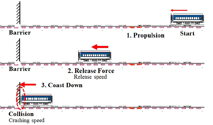
2.2 Test Phases

Basically, the whole testing process in a typical real train collision test can be

divided into two major phases, propulsion phase and coast-down phase. In

propulsion phase, a test vehicle is pulled by a propulsion cart and accelerated on the

guided track to a designated high speed in a very short time and then the test vehicle

is released from the propulsion cart. From this time on, since the test vehicle is

separated from the propulsion cart, it will coast down towards the rigid wall (or a

barrier) and hit the rigid wall eventually. The crash speed is measured accurately

which is one of the most important indicators for the whole testing. For some special

purposes, a barrier (e.g. a car) will be placed close to the rigid wall and to be crashed

into the test vehicle.

Under the real test conditions, the test vehicle is not released right away when

it reaches the designated speed, it will maintain a certain speed for some time and

get released at designated location and speed. In this paper, we only discuss the

(33)

and location. In Figure 2.5, it shows that the test vehicle is started from the

right-hand side along a guided track. It will be propelled to a certain speed to release the

propulsion force. After the propulsion force is released, the test vehicle will coast

down towards the barrier (losing speed because of the resistance force), which could

be a rigid wall or a car. The crash speed is the speed, at which the test vehicle hits

the barrier. The crash speed is a very important indicator for test facilities in this

industry and it will be measured according to industry standard.

Figure 2.5 Propulsion – Release Force – Coast Down.

2.3 Test Facility

A real train collision test could be a train to truck or car, train to a rigid wall or

train to train. In the test facility involved, it will be train to rigid wall and train to

(34)

Figure 2.6 Train and Track. Source: Anemoi Technologies Inc.

The rigid wall is built inside a building with well-designed protection facilities.

The building is shown in Figure 2.7 which is located at the other end of the track.

And in Figure 2.8, it shows the rigid wall inside the building. This rigid wall is built

with huge concrete base designed for high-speed collision test.

Figure 2.7 Building Housing the Rigid Wall. Source: Anemoi Technologies

Inc.

(35)

The whole testing process will be done in about 15 to 30 second. A powerful

electric motor and a specially-made pulling drum will be used in providing the

propulsion force. A powerful braking drum will also be used to brake the propulsion

system or the vehicle after the release, in the case of emergency. The highest required

crash speed in the test facility in this research is a record high of 150kph for a

15000kg vehicle.

2.4 Vehicle Motion Analysis

During the propulsion phase, a test vehicle needs to be propelled on a straight,

guided track, to a particular speed 𝑉𝑟 (release speed), at which time the test vehicle

is released to coast down towards a barrier where it is required to crash at a speed of

𝑉𝑐 (crash speed). The distance between the start of the propulsion and the crash

barrier is known. The difference between 𝑉_𝑟 and 𝑉_𝑐 is dependent on the

coast-down distance (which itself is dependent on where the test vehicle is released from

the propulsion mechanism) and the resistance forces during the coast-down, such as

friction (both between wheels and rail and also train-internal friction such as bearing

frictions etc.) and aerodynamic force.

In general, the equation of motion is

𝐹 − 𝑅 = 𝑀 ∗ 𝐴, (2.15)

where 𝐹 is the propulsion force, 𝑅 is the resistance force, 𝑀 is the mass of

vehicle, and 𝐴 is the vehicle acceleration. Mass 𝑀 can be measured and it is

constant. Propulsion force 𝐹 is controlled and measured. The propulsion

acceleration 𝐴 changes but it can be measured during the propulsion phase.

Resistance force 𝑅 is the sum of friction and aerodynamic force. Friction is

constant which can be defined by coefficient of friction and mass. Aerodynamic

force 𝑅ae can be defined as follows

𝑅_ae = 𝑐𝑣 +1

2𝑆𝜌𝐶𝑑𝑣², (2.16)

(36)

density, 𝐶_𝑑 is train drag coefficient and 𝑣 is the speed. Because we do not know

in advance what those parameters in equation (2.16) are, such as 𝜌, 𝐶_𝑑,etc., it is

impossible to obtain the value of 𝑅_ae by using equation (2.16). But by observing

equation (2.15), when 𝐹, 𝑀 and 𝐴 can be measured, the resistance 𝑅 is the only

unknown variable and can be calculated by equation (2.15). This is the fundamental

reason why regression analysis is needed in this research. And the knowledge of how

to use multiple linear regression analysis model to deal with the quadratic

relationship between dependent variable and independent variables is already

introduced in Section 2.1.3.

For the coast-down movement, since the propulsion force is released,

𝐹 = 0.

Because resistance 𝑅 has the quadratic relationship with speed 𝑣, the regression

function of resistance 𝑅 can be expressed in a general form as follows,

𝑅 = 𝑏0+ 𝑏1𝑣 + 𝑏2𝑣², (2.17)

where 𝑏0, 𝑏1, 𝑏2 are regression coefficients. According to equation (2.15) and

(2.17), we have

𝐴 = 𝑑𝑣

𝑑𝑡= − 𝑅 𝑀= −

(𝑏₀+𝑏₁𝑣+𝑏₂𝑣²)

𝑀 . (2.18)

Therefore, for coast-down movement, the acceleration 𝐴 can be calculated by

equation (2.18) once regression coefficients 𝑏₀, 𝑏₁ and 𝑏₂ are determined.

Thus, during the propulsion phase, speed 𝑣, propulsion force 𝐹 and

acceleration 𝐴 need to be measured so that the actual propulsion performance could

be continually extrapolated over a very short time. Based on the performance data

(speed 𝑣 , acceleration 𝐴 and propulsion force 𝐹 ) collected, the value of resistance

force 𝑅 can be calculated using equation (2.15). The values of speed 𝑣 and

resistance force 𝑅 form a set of data, {(v, R)}, describing the relationship between

speed 𝑣 and resistance force 𝑅. Then, following the discussion of regression

analysis model in Section 2.1, the quadratic regression analysis model will be

(37)

and speed 𝑣 is the independent variable. By applying the least squares method

discussed in Section 2.1.3 and 2.1.4, the regression coefficients 𝑏₀, 𝑏₁, 𝑏₂ in

equation (2.17) can be calculated and determined. Then the regression function of

𝑅 is determined. This resistance function 𝑅 is critical in the simulation of

coast-down movement and the calculation of release speed and location.

2.5 Sample Data Sheet

Figure 2.9 Sample Data 1. Source: Anemoi Technologies Inc.

Figure 2.9, part of the sample data sheet, is provided by Anemoi Technologies

Inc. This data set is used in the design stage to estimate and simulate the propulsion

performance, such as propulsion force, speed and acceleration, in order to better

design the whole mechanism. In the real test facility, the propulsion performance

data will be collected in a real time manner using sensors. There are 209 rows of

records in this data sheet from the speed of zero to speed of 150kph.

(38)

calculated. Actual data is the one output from the propulsion system, or the data

applied in theory. It can’t be obtained exactly in reality due to mechanical

deviations. Measured data is the one collected from the sensors placed along the

track or installed on the propulsion cart. Calculated data is the one by calculation

based on other known data. The columns in this data sheet are 𝑣 of speed, 𝐹𝑎 of

actual force, 𝐹𝑚 of measured force by sensor, 𝑅𝑎 of actual resistance, 𝐴𝑎 of

actual acceleration, 𝐴_𝑚 of measured acceleration by sensor and 𝑅_𝑐 of

calculated resistance.

Figure 2.10 shows another part of sample data sheet which explains the formula

to estimate actual force 𝐹_𝑎, measured force 𝐹_𝑚, actual resistance 𝑅_𝑎, actual

acceleration 𝐴_𝑎, and measured acceleration 𝐴_𝑚.

Figure 2.10 Sample Data 2. Source: Anemoi Technologies Inc.

As shown in Figure 2.10, 𝐹_𝑎, cell 𝐷₈, is simulated by a quadratic function of

speed 𝑣 , the expression of 𝐹𝑎 can be written as

𝐹𝑎= 𝑐0+ 𝑐1𝑣 + 𝑐2𝑣², (2.19)

where 𝑐0, 𝑐1and 𝑐2 are coefficients. The value of 𝑐0, 𝑐1and 𝑐2 are set in the cell

𝐷₃, 𝐷₄ and 𝐷₅. Considering the mechanical deviations between the actual and

measured data, the value of 𝐹_𝑚, cell 𝐸₈, is the addition of 𝐹_𝑎 and variance of

errors, following the equation

𝐹_𝑚 = 𝐹_𝑎− 𝑀𝑎𝑥(𝐹_𝑎) ∗ 𝐸1+ 2 ∗ 𝑅𝐴𝑁𝐷() ∗ 𝑀𝑎𝑥(𝐹𝑎) ∗ 𝐸1, (2.20)

where 𝐸₁ is an error ratio for 𝐹_𝑎 that is used to describe the noise of initial

(39)

is ranged from 0 to 1, and 𝑀𝑎𝑥(𝐹_𝑎) is the maximum value among all the data values

of 𝐹_𝑎. According to the sample data provided in Figure 2.10, 𝑅_𝑎, cell 𝐹₈, is also

estimated by using a quadratic function of speed 𝑣, its expression can be written as

𝑅_𝑎 = 𝑑₀𝑀𝐺 + 𝑑₁𝑀𝐺𝑣 + 𝑑₂𝑣², (2.21)

where 𝑑0, 𝑑1and 𝑑2 are coefficients, M is the mass of test vehicle, and G is the

gravity acceleration (G=9.81). The value of 𝑑0, 𝑑1 and 𝑑2 are set in the cell

𝐺2, 𝐺3 and 𝐺4. The value of M is set in the cell 𝐺5. According to equation (2.15),

the actual acceleration 𝐴_𝑎, cell 𝐺₈, can be obtained by

𝐴𝑎 = 𝐹𝑎−𝑅𝑎

𝑀 . (2.22)

The value of 𝐴_𝑚, cell 𝐻₈, is the addition of 𝐴_𝑎 and variance of errors, following

the equation of

𝐴𝑚 = 𝐴𝑎(1 − 1

2𝐸2+ 𝑅𝐴𝑁𝐷()𝐸2), (2.23)

where 𝐸₂ is an error ratio for 𝐴_𝑚 with its value set in the cell 𝐻₆. The value of

𝑅𝐴𝑁𝐷() is ranged from 0 to 1 as well.

The last field, cell 𝐼₇, in the sample data sheet of Figure 2.10 is 𝑅_𝑐, the

calculated resistance force. According to equation (2.15), 𝑅_𝑐 can be obtained

by

𝑅_𝑐 = 𝐹_𝑚− 𝑀 ∗ 𝐴_𝑚. (2.24)

Eventually, after implementing the logic and formulas in the developed software

based on the data sheet of Figure 2.9 and Figure 2.10, a data set of pairs of speed 𝑣

and 𝑅_𝑐, {(𝑣, 𝑅_𝑐)} , is obtained which describes the characteristics of the relationship

between speed and resistance force. This data set {(𝑣, 𝑅_𝑐)} will be applied later on

to determine the regression coefficients for a fitted regression function that can be

used to predict the behavior of resistance force.

In this research, the actual data is used only to help estimate the measured data,

so that a simulated data set can be generated. In the real collision test environment,

the measured data will be obtained from various sensors. In the following sections

(40)

as 𝐹_𝑎, 𝐹_𝑚, 𝐴_𝑎 and 𝑅_𝑐, are no longer used. Only the capital letter will be used to

express the measured value or the calculated value for each variable. For example,

𝐹 means the measured force, 𝑅 means the calculated resistance, 𝐴 means the

measured acceleration and 𝑀 means the measured mass.

(41)

Chapter 3 Proposed Solution -

RTPSA

In this chapter, details of the proposed approach will be introduced. The

software developed is called 𝑅𝑇𝑃𝑆𝐴 – Real Time Predictive Speed Analysis.

3.1 Limitation of Existing Methods

In a real collision test facility, the propulsion system is the key component. It is

a group of mechanical and electrical machinery and equipment and it needs to be

calibrated before putting it into operation. To-date such calibration was based on

theoretical data and past experience. But during the test, resistance forces, such as

friction resistance force and aerodynamic resistance force, play an important role

influencing the behavior of test vehicle movement. Resistance forces vary all the

time and are subject to the speed of test vehicle, wind speed and direction,

temperature and humidity. So every test is different. When the propulsion system is

calibrated using old data or parameters, it leads to less accuracy in terms of the

release speed and location, and the crash speed as well. The essence of 𝑅𝑇𝑃𝑆𝐴 is

that the most up-to-date calibration information can be derived from studying in real

time the actual propulsion behavior during the actual test. In order to do this, an

efficient algorithm needs to be in place to calculate and predict the movement

behavior of test vehicle during propulsion. This algorithm also needs to work in a

real-time manner to monitor and control all the activities along the test.

3.2 Objective

The proposed approach in this research work is to address the issues discussed

(42)

by implementing a new design for a real collision test facility. A simulated data set

is generated and used to describe the performance in propulsion phase. The quadratic

regression analysis model is applied in this implementation to predict the behavior

of resistance force and simulate the movement of the test vehicle. The proposed

software works in a real-time manner and provides a more accurate release location

and speed for the overall control system to fulfill the actual force release.

3.3 Design Principles

There are three design principles for the proposed approach in this thesis. They

are real-time, predictive, and simulation.

3.3.1 Real-Time

During the propulsion phase, the propulsion performance (speed, acceleration

and propulsion force) are measured on a real-time basis, instead of using old data

and past experience, so that the actual performance could be continually extrapolated

in a very short period of time. This lets the software calculate the regression

coefficients 𝑏0, 𝑏1, 𝑏2for resistance function (2.17) by inserting this into equation

(2.15) and measuring 𝐹 and 𝐴 (𝑀 is known). And this approach leads to better

accuracy in the prediction of resistance force behavior which is the key factor

influencing the overall performance.

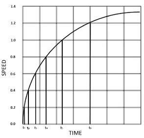
In this research work, a data set (stream) is generated simulating the behavior

of propulsion phase in a real-time manner. When generating the simulated data

stream, as shown in Figure 3.1, the whole propulsion phase is divided into many

small intervals of speed. The X-axis in Figure 3.1 is time and Y-axis is speed. Each

interval has the same speed difference of 0.2m/s. For each of the small speed

(43)

resistance 𝑅 (Eq. (2.24)) are all calculated following the rules and formulas

discussed in Section 2.5.

Figure 3.1 Small Intervals of Propulsion Curve

Meanwhile, each small interval is treated as constant acceleration motion. By

applying the constant acceleration motion formulas, the time length, distance and

location can be calculated. For example, for interval 𝑖 , let 𝑣i0 denote the start speed,

𝑣it denote the end speed, 𝐴 denote the acceleration, 𝑡 denote the time spent, 𝑆𝑖0

denote the start location, and 𝑆_𝑖𝑡 denote the end location, then

𝑣_it= 𝑣_i0+ 𝐴𝑡, (3.1)

𝑆_𝑖𝑡 = 𝑆_𝑖0+ 𝑣_i0𝑡 +1

2𝐴𝑡². (3.2)

From equation (3.1), we have

𝑡 =𝑣it− 𝑣i0

𝐴 . (3.3)

Since 𝑣_it and 𝑣_i0 are known for each interval, and acceleration 𝐴 can be obtained

by equation (2.23), so from equation (3.3), time 𝑡 can be obtained. By substituting

(44)

Eventually, a data set of details of propulsion performance is obtained after the

calculation. Specifically, a data set {(𝑣, 𝑅)} of pairs of speed 𝑣 and resistance 𝑅

is obtained which describes the characteristics of the relationship between speed and

resistance force. This data set of speed and resistance {(𝑣, 𝑅)} will be applied later

on to determine the regression coefficients for a fitted regression function that can

be used to predict the behavior of resistance force. In conclusion, the whole

propulsion phase is monitored and described in detail. The design of small interval

makes it possible to monitor the whole propulsion behavior in a real-time manner.

3.3.2 Predictive

The prediction capability in 𝑅𝑇𝑃𝑆𝐴 software is based on the real-time

performance data that comes from the propulsion phase. One of the results of

simulated data stream is a data set of pairs of speed 𝑣 and resistance force 𝑅,

{(𝑣, 𝑅)}. As discussed in Section 2.4, 2.5 and 2.1.3, resistance force 𝑅 has the

quadratic relationship with the speed 𝑣 and multiple linear regression model can be

applied to the quadratic relationship after the substitution of independent variables.

The general form of the fitted regression function can be written as

𝑅 = 𝑏₀+ 𝑏₁𝑣 + 𝑏₂𝑣², (3.4) same as (2.17)

where 𝑏₀, 𝑏₁, 𝑏₂ are regression coefficients. By applying the least squares method

introduced in Section 2.1.4 into the data set {(𝑣, 𝑅)}, the regression coefficients

𝑏₀, 𝑏₁, 𝑏₂ are calculated. With the determination of regression coefficients 𝑏₀, 𝑏₁, 𝑏₂,

the fitted regression function of resistance 𝑅 (Eq. (3.4)) will be used to predict the

equation of motion during the coast down period, as well as for the last period of

propulsion phase. Details of the simulation for the last period of propulsion phase

will be introduced in section 3.3.3 and 3.9.

As discussed earlier, resistance force 𝑅 plays an important role in the whole

test phases. With the in-time prediction of resistance force 𝑅, details of the behavior

(45)

that makes it possible to calculate and find the release speed and location.

3.3.3 Simulation

Simulation technique is needed and implemented in 𝑅𝑇𝑃𝑆𝐴 because the

algorithm needs to be triggered to calculate and provide the release location and

speed to the control system before the test vehicle actually reaches the release point.

A leading time of 1-2 second is required for the control system to activate the actual

force release. Simulation is a practical way to do this work.

There are two movement phases that need to be simulated in order to figure out

the release location and release speed, the last period of propulsion and the

coast-down movement.

Figure 3.2 Start and End Points for Simulations. F: Calculate Regression Coefficients; G: Use Regression Coefficients to Calculate Coast-down Behavior

Backwards

As shown in Figure 3.2, the 𝑋-axis is location while the 𝑌-axis is velocity. The

(46)

𝐵 the propulsion force is released and the coast-down phase starts at position 𝐵

right away. Position 𝐷 is the end of coast-down movement where the test vehicle

hits the barrier. During propulsion, when test vehicle reaches position 𝐶, the

algorithm is used to calculate the release location and release speed. The movement

from 𝐶 to 𝐵 is called the last period of propulsion in this research. By observing

Figure 3.2, point 𝐵 is the release point and it is the intersection of 𝐶𝐵 and 𝐵𝐷.

Therefore, in order to figure out the release location and release speed at position 𝐵,

the function of line 𝐶𝐵 and the function of line 𝐵𝐷 must be known. Simulation

technique is the choice in this research. With the simulation of movements of

coast-down 𝐵𝐷 and the last period of propulsion 𝐶𝐵, it becomes possible, at position 𝐶,

to calculate the release location and release speed.

Details on how to do these two simulations are introduced in Section 3.8.1 and

Section 3.9.1.

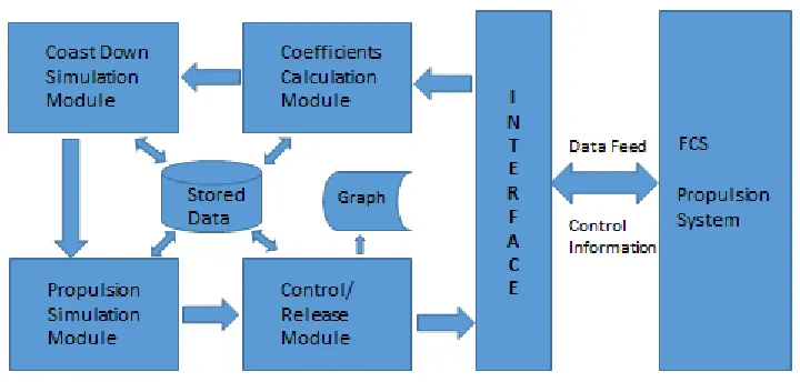
3.4 System Architecture

In a real test facility, physically, there are an array of sensors to measure the

performance, such as propulsion force, acceleration, speed, location, temperature,

humidity, wind speed and direction. They are installed on the propulsion cart which

pushes the test vehicle, along the guided track and in the building. Sensors are

connected to an IP network and controlled by an overall control system, which is

called Facility Control System (FCS). PLC (Programming Logic Controller)

controllers and DeviceNet/Ethernet converters are also used to help convert signals

and do the preliminary calculation. Figure 3.3 shows an overall system architecture

(47)

Figure 3.3 System Architecture. Source Anemoi Technologies Inc.

In Figure 3.3, the Facility Control System (FCS) is the core which is installed

in a database server located at top left of the figure. All the activities are controlled

by FCS. Data interface is designed and used by FCS to collect real-time data from

sensors, PLCs and VFD (Vary Frequency Device). Command interface is designed

and used by FCS to send control command to PLCs, VFD and sensors. All the

equipment, such as DB server, main control monitors, administrative work stations,

VFD, PLC controllers and many different sensors, are connected in a high speed

Ethernet network. Most of the sensors are connected into Ethernet through PLCs.

Some special sensors are connected through Ethernet converters, such as radar speed

sensor and laser distance sensor. 𝑅𝑇𝑃𝑆𝐴 is part of FCS and used to collect the

performance data in a real-time manner from sensors during propulsion phase and

provide input to FCS to actually control the force release.

3.5 Software Structure

The 𝑅𝑇𝑃𝑆𝐴 software works in a real-time manner. It has a main process and

four modules.

Real Time Predictive Speed Analysis for High Speed Rail Collision Test

Scholarship at UWindsor

Scholarship at UWindsor

Real Time Predictive Speed Analysis for High Speed Rail Collision

Real Time Predictive Speed Analysis for High Speed Rail Collision

Test

Test

Real Time Predictive Speed Analysis for High

Speed Rail Collision Test

Author’s Declaration of Originality

Abstract

Dedication

Acknowledgements

TABLE OF CONTENTS

LIST OF TABLES

LIST OF FIGURES

Chapter 1 Introduction

1.1 Introduction of High Speed Rail

1.2 Brief History of HSR

1.3 Safety Issues and Technology

1.4 Motivation

1.5 Contributions

1.6 Guide to the Thesis

Chapter 2 Background Knowledge

2.1 Regression Analysis

2.1.1 Simple Linear Regression

2.1.2 Multiple Linear Regression

2.1.3 Quadratic Relationship between Dependent and

Independent Variables

2.1.4 Calculation of Regression Coefficients

2.1.5 Correlation Coefficient -

R

²

2.2 Test Phases

2.3 Test Facility

2.4 Vehicle Motion Analysis

2.5 Sample Data Sheet

Chapter 3 Proposed Solution -

RTPSA

3.1 Limitation of Existing Methods

3.2 Objective

3.3 Design Principles

3.3.1 Real-Time

3.3.2 Predictive

3.3.3 Simulation

3.4 System Architecture

3.5 Software Structure