An eye-tracking study on synonym replacement
byCassandra Svensson
LIU-IDA/KOGVET-G--15/005--SE
Supervisor : Arne J¨onsson
Dept. of Computer and Information Science
at Link¨oping University
Examiner : Mathias Broth
Dept. of Culture and Communication at Link¨oping University
simplification also increase. There are some strategies for doing that and this thesis has studied two basic synonym replacement strategies. The first one is called word length and is about always choosing a shorter synonym if it is possible. The second one is called word frequency and is about always choosing a more frequent synonym if it is possible. Three different versions of them were tried. The first one was about just choosing the shortest or most frequent synonym. The second was about only choosing a synonym if it was extremely shorter or more frequent. The last was about only choosing a synonym if it met the requirements for being replaced and was on synonym level 5. Statistical analysis of the data revealed no significant difference. But small trends showed that always choosing a more frequent synonym that is of level 5 seemed to make the text a bit easier.
Keywords : Synonym replacement, word lenght, word frequency, eye tracking
number of people. I would especially like to thank my enthusiastic and inspiring supervisor Arne J¨onsson for constantly being available to support me and believing in me. I would like to thank Evelina Rennes for sharing her experience with the eye tracker and support-ing me dursupport-ing that stage in the project. For givsupport-ing helpful comments on the text during its final stage, I would like say thanks to Lovisa Jansson. I would also like to thank Mathias Broth my examiner, and the rest of my supervisor group for great and useful feedback during the all group seminars. I am thankful to all that participated in the study, without them the study would not have been possible.
A final thanks goes to my love Daniel Fahl´en for supporting me during the whole process of writing this thesis.
List of Tables vii List of Figures ix 1 Introduction 1 2 Background 4 2.1 Reading . . . 4 2.2 Eye-tracking . . . 6 2.2.1 Fixation Duration . . . 7 2.2.2 Number of fixations . . . 8 2.2.3 Pupil Size . . . 9 2.3 Semantic Relations . . . 9 2.3.1 Synonymy . . . 9 2.3.2 Synonym Replacement . . . 10 2.4 Readability . . . 11 2.5 Language resources . . . 12 3 Method 14 3.1 Research design . . . 14 3.2 Participants . . . 15 3.3 Material . . . 15 iv
3.3.1 Equipment . . . 16 3.3.2 Stimuli material . . . 16 3.3.3 Reading order . . . 19 3.4 Data Collection . . . 20 3.5 Data analysis . . . 21 4 Results 24 4.1 Readability metrics . . . 24 4.1.1 LIX . . . 25 4.1.2 OVIX . . . 26 4.2 Experiment 1 . . . 27 4.2.1 Fixation Duration . . . 27 4.2.2 Number of fixations . . . 28 4.2.3 Pupil size . . . 29
4.3 Experiment 2: Extreme synonyms . . . 31
4.3.1 Fixation duration . . . 31
4.3.2 Pupil size . . . 32
4.4 Experiment 3: Synonym level 5 . . . 34
4.4.1 Fixation duration . . . 34 4.4.2 Pupil size . . . 35 5 Analysis of results 38 5.1 Readability metrics . . . 38 5.2 Experiment 1 . . . 39 5.2.1 Fixation duration . . . 40 5.2.2 Number of fixations . . . 40 5.2.3 Pupil size . . . 41
5.3 Experiment 2: Extreme synonyms . . . 42
5.3.1 Fixation duration . . . 42
5.3.2 Pupil size . . . 43
5.4 Experiment 3: Synonym level 5 . . . 43
5.4.2 Pupil size . . . 44
6 Discussion 46
6.1 Procedure . . . 46 6.2 Results . . . 47
7 Conclusion 50
A Text B - Original version 53
B Text B - Word length version 56
C Text B - Word frequency version 59
D Text B - Used synonym candidates 62
3.1 The table shows the number of synonym replacements, (and in parentheses the percentage), performed per text. O shows how many words that met the require-ments to be replaced while the L and F show how many words that actually were replaced in each text.
The percentage on ”same” is counted on all O words. . 19 3.2 The table shows the different combination in which
the text were presented. . . 20 4.1 LIX-value on all three versions of the three texts and
respective mean value. . . 25 4.2 OVIX-value on all three versions of all three texts and
respective mean value. . . 26 4.3 The table shows the mean and standard deviation for
the groups that have been compared. . . 27 4.4 The table shows the mean and standard deviation for
the groups that have been compared. . . 29 4.5 The table shows the mean and standard deviation for
the groups that have been compared. . . 30 4.6 The table shows the mean and standard deviation for
the groups that have been compared. . . 32
4.7 The table shows the mean and standard deviation for
the groups that have been compared. . . 33 4.8 The table shows the mean and standard deviations for
the groups that have been compared. . . 35 4.9 The table shows the mean and standard deviation for
2.1 Formula for LIX. . . 12 2.2 Formula for OVIX. . . 12
Introduction
The field of automatic text simplification has grown a lot over the last 20 years. The reason for this is partly because there is probably an increased need for it as the amount of information grows. Chan-drasekar et al. (1996) writes about some of the reasons why they thinks text simplification is important. Firstly, because syntacti-cally complex sentence and ambiguities are likely to generate a large number of parses which can cause parsers to fail. Chandrasekar et al. (1996) thinks that the parsers of simpler sentences may improve the quality of machine translation.
Information retrieval systems usually get large segments of text of where only a part may be relevant. Chandrasekar et al. (1996) mean that with simplified texts it should be possible to extract specific phrases or simple sentences of relevance in response to queries. Peo-ple faces an overload of information today, Chandrasekar et al. (1996) mean that it would be helpful to have summarization tools that use simplification to weed out irrelevant parts out of a large text. An-other reason is that modern computers allow it with all natural
guage processing tools and corpora.
To do a simplification manually by hand is very time consuming and very expensive. Therefore we need an automated method that can be trusted when it comes to important documents. The task of automatic text simplification consists among other things of being able to find and replace difficult words with more simple ones, with-out altering or changing the meaning of the text. This can be done by replacing more difficult words with one of its simpler synonyms. The question is how this synonym should be selected.
Keskis¨arkk¨a (2012) did a study on automatic lexical simplification via synonym replacement in Swedish. He investigated three differ-ent strategies for choosing synonyms; based on word frequency, word length and level of synonymy. The strategies were evaluated by stan-dardized readability metrics for Swedish. His result showed that re-placement based on word frequency and word length can improve readability in terms of established metrics but that the risk of intro-ducing errors in the text is high.
Skeppstedt and Kvist (2014) did a study partly based on Keskis¨arkk¨a (2012) where they wanted to replace specialised medical terms with easier synonyms. By easier they meant more frequent. The results were evaluated by established metrics which showed that the easier terms were longer, resulting in that one of the values increased while the other value decreased a little bit.
The aim of this study was to investigate how to select satisfying synonym candidates with two simple synonym replacement strate-gies as a base. This was done by investigating how choosing more frequent synonyms and shorter synonyms affect reading behaviour. This was explored by tracking the participants eye movements
dur-ing the readdur-ing of different texts with an eye trackdur-ing camera.
The main questions of the study were:
• How is the reading affected when texts are simplified by having synonyms replaced based on word length or word frequency?
• Does a text become easier to read when synonyms are replaced based on word length and word frequency?
• How does level of synonymity and extremely short or frequent synonyms affect the results?
Background
This chapter presents a brief overview of the theoretical background that concerns this study. To begin with is reading as a mental pro-cess explained in section 2.1. Then eye-tracking and three different measurements are explained in section 2.2. Semantic relations, syn-onymity and synonym replacement are explained in section 2.3. In section 2.4 readability and two different readability measurement are explained. Last in section 2.5 the used language resources are ex-plained.
2.1
Reading
Reading is a very complex mental process that is both top-down and bottom-up. The first step is to recognize letters. The letters can be presented in many different ways when it comes to type styles and typefaces, and they may also be in capital or lower case form. The fact that we can recognize the same letter when it is presented in dif-ferent type styles and typefaces can be explained by the recognition-by-components theory, which indicates that reading is a bottom-up
process. Then when you know which letter you are looking at, you need to translate that letter into a sound. These sounds need to be split up into sequences to form words. The breakdown of the sounds into words can be said to be a top-down process because here you get help from the context and your prior experience of reading. When you have identified a word you just need to figure out what that word means. And when you are done, you just repeat the process until you are done reading.
According to Morton (1969) one important aspect of reading is lexi-cal access. It is not until we have recognized a word that we can un-derstand the meaning of the word from our memory. It is a common assumption that lexical access is an interactive process that com-bines information such as the feature of letters, letters themselves and the words comprising the letters. Plaut et al. (1996) explains that the reason this is called interactive is because this view implies that besides visually perceptible features we also use the features we already know about the words to identify letters. Nation and Snowl-ing (1998) thinks this hypothesis can be characterized as a “division of labour” between a phonological process that deals with mappings between orthographic (e.g.spelling) and phonological (e.g. sounds in languages) representations and an interacting semantic process which deals with mappings between semantic, phonological, and or-thographic representations. Nation and Snowling (1998) describes these two processes as the phonological pathway and the semantic pathway.
Semantic priming according to Neely et al. (1989) describe how indi-viduals react faster to a target word when preceded by semantically related words, compared with unrelated ones. An example of this is given in a study by Becker (1980), where it was shown that a word is processed faster if it is followed by semantically related words
com-pared to when the relationship between the prime words and target words is unrelated or neutral. Faster availability of lexical informa-tion is said to be explained by the participants assumed to create an expectation of words that are likely to follow the prime word. When the target word matched the expectation created by the prime word, the participants’ reaction time decreased at a lexical decision task where they had to decide whether stimuli were words or non-words. This expectation can be explained as so-called spreading activation, which according to Traxler et al. (2000) involves activation of a word in an individual’s mental lexicon that spread to related words and thereby causes priming. Because the words doctor and nurse often occur together there is a strong link between them where activation can spread, and doctor may therefore be a likely priming for nurse, or vice versa. Thus, Traxler et al. (2000) believes that context improves processing of new words when the activation of these increases as a result of previously encountered words with related meaning.
2.2
Eye-tracking
To study mental processes like reading, eye-tracking can be used. Irwin (2004) writes that the eye position may seem to be an ideal dependent variable because eye movements are a natural and fre-quent behavior but there are some problems that he presents. The first one is that the locus of cognitive processing may include more than just the fixation location. The second one is that the locus of cognitive processing can be dissociated from the fixation location. The third problem is that the eye position is not always under cog-nitive control. And the last problem is that cogcog-nitive processing can occur during eye movements as well as during eye fixations. But de-spite this, Duchowski (2007) means that monitoring eye movements
is a good and well tried way to study cognitive processes in reading.
2.2.1
Fixation Duration
Fixation duration is the time that the eye is fixed at some point. Holmqvist et al. (2011) says that the word ”fixation” is a bit mis-leading because the eye is not completely still, it makes different typs of micro-movements all the time and that a typical fixation is 200-300 ms long. Fixation duration is calculated by fixation detec-tion algorithms that do not care about the visual intake. The eyes always make micro-movements, and a fixation is therefore defined as a point with a certain radius within which the micro-movement takes place. This means that, depending on the settings that are used, what counts as fixation duration will vary. Holmqvist et al. (2011) also writes about the importance that the data is of good quality. If there is smooth pursuit, the data will give you faulty fix-ation durfix-ations.
Because the average fixation duration varies depending on how the task and stimuli are designed, it is important to be careful when designing the texts so that they are as similar as possible. Factors like stress might result in shorter fixations; therefore it is important that the participants retain the same level of stress during the whole test. There are a few known problems with this measuring method but they apply mainly to studies involving picture perception, visual search, and everyday vision, and not so much for reading studies (Irwin, 2004).
According to Holmqvist et al. (2011), it could be argued that fixation duration measures how much effort is needed for the cognitive pro-cessing of a text. A complicated text needs more cognitive propro-cessing while an easier text needs less. Dambacher and Kliegl (2007) have
shown that longer fixation durations correlate with larger N400 am-plitudes, which is considered to be indicative of the fact that meaning and semantic content are being processed. Raney and Rayner (1995) have shown that words that are less frequent and therefore require a longer lexical activation process, generally generates longer fixation durations. A complicated text or texts with complicated grammar also gives rise to longer fixation durations.
2.2.2
Number of fixations
The number of fixations measure how many fixations a person does within a specific area or on a whole text. The number of fixations can refer to an entire trial, such as reading one page or to the num-ber of fixation in a area of interest (AOI). According to Holmqvist et al. (2011) it is important when using number of fixations that the space of which the stimuli takes up and the time the participants can spend looking at the stimuli are as equal as possible. When the trial time is constant, it shall also be an inverse relationship between number of fixation and fixation duration.
According to Holmqvist et al. (2011), the number of fixation is usually used as an indication of many different things, for exam-ple to show the semantic importance. Loftus and Mackworth (1978) showed that significantly more fixations landed on semantically infor-mative areas. Another example is in reading were number of fixations is used as a measure of morphological complexly, word frequency and familiarity (Clifton et al., 2007). The theory says that in an area of interest containing a long or unfamiliar word shall receive more fix-ations than a short and familiar word.
2.2.3
Pupil Size
Hess and Polt (1964) showed that the size of the pupil increased during problem solving. They claimed that it seemed evident that the pupil response is a direct reflection of neurological activity. They saw that the pupil size increased in correlation to the difficulty of the task and therefore thought that it could be used as a measurement for cognitive activity. The pupil size is measured in pixels and is measuring by the horizontal diameter because the vertical diameter is too sensitive to the eyelid closing.
Holmqvist et al. (2011) writes that when using pupil size as a mea-surement of cognitive states, it is important to remember that the cognitive effects on the pupil are small. They can therefore easily be smoothed out if, for example, the light in the room changes.
2.3
Semantic Relations
Semantics is the study of word meaning. The meaning of words can have different relations to each other, which are called semantic rela-tions. There are a few different semantic relations but according to Jurafsky and Martin (2009) the most common ones used in computa-tional investigations are synonymy (similar), anatonymy (opposite) and hypernymy (subordinate). Synonyms can be used to make texts easier to read. Anatonymys can be used to explain the meaning of a word in a lexicon and a hypernymy is usually used to explain other word in a thesaurus.
2.3.1
Synonymy
A common explanation of synonyms is that they are words that can replace each other in some class to contexts with insignificant change
of the whole text’s meaning. Ingo (2011) thinks it is important to keep in mind that words can be synonyms, but have very different shades of meaning, stylistic features or connotations. He argues that this is important to consider when a new synonym is chosen to re-place another. This is because depending on what synonym is chosen, a sentence can completely change its meaning. Bolshakov and Gel-bukh (2004) talks about absolute and non-absolute synonyms. They say that if two words can replace each other in any context without any change in meaning, these are absolute synonyms. One example that they mention is sofa and settee but these types os synonymes are extremely rare in any language.
2.3.2
Synonym Replacement
Three common methods for synonym replacement are word frequency, word length and level of synonymy. Word frequency can be calcu-lated in several different ways. One option is to choose the most commonly used word in a corpus. Another alternative is to choose the most frequent word based only on texts that are similar to the original text. Another possibility is to choose the most frequent word based on the text’s own contexts. If this is done, it is considered to improve the readability of the text Raney and Rayner (1995) because the reader probably has come across the word many times before. A word’s length can be an indicator of how difficult a word is, and many readability metrics take into account word length. Therefore, if words are replaced with shorter synonyms, the text’s estimated difficulty will be lower. Under this assumption, you can then change a text’s difficulty by replacing synonyms composed of many letters with synonyms with fewer letters. Level of synonymy is about choos-ing the synonym with the maximum score in relation to the current word.
2.4
Readability
According to Lewis et al. (1986), readability as a concept and as an area of research, has been characterised by a variety of definitions, and number of measurement formulae. Readability is concerned with studying the problem of matching the reader with a text and evalu-ate how easy the text is to read. Heimann M¨uhlenbock (2012) writes that to achieve readability the vocabulary used and the syntactical structure must correspond to the reading stage of the individual. One other aspect that she thinks is important is that the readers de-coding skills are developed to a certain degree in order to master the challenge of reading unknown words and that the reader has prior knowledge of the topics in the text. Things that are assumed to af-fect the readability are word frequency and word length (Rello et al., 2013). They did a study on how word frequency and word length affected people with and without dyslexia. The results showed that the time it took to read the texts and the participants fixation du-ration became shorter for both word frequency and word length but only for the participants with dyslexia. For the participants without dyslexia there were no differences at all.
A number of readability metrics have been developed to study the readability of a text. The most established readability metrics for Swedish texts are LIX and OVIX. LIX stands for readability index. LIX was from the beginning intended to assess readability across lan-guages and Lewis et al. (1986) predicted already back then that LIX had the potential to act like reliable predictor of readability assess-ments. Now is it the most common readability metric for Swedish texts. LIX takes into account the number of words, number of sen-tences and the number of long words (>6 characters). A simple text gets a value between 25 and 30; a normal text gets a value between 30 and 40 while research and theses usually end up at a value above
60. The formula for calculating LIX is presented in Figure 2.1.
LIX = number of words
number of sentences+
number of words > 6 characters
number of words ×100
Figure 2.1: Formula for LIX.
OVIX stands for word variation index and involves calculating lexi-cal variation. A high value usually indicates a low readability value. OVIX takes into account the number of words and the number of unique words. The formula for calculating OVIX is presented in Fig-ure 2.2.
OV IX = log(number of words) log
2− log(number of words unique words)
log(number of words)
Figure 2.2: Formula for OVIX.
2.5
Language resources
The sections below describe the resources that have been used in the study. SynLex was used to find synonym candidates on the right level. SUC 3.0 was used to get the frequency of the synonym can-didates. SynLex is a synonym dictionary containing 38,000 Swedish synonym pairs. This resource was developed at KTH by allowing the
users of Lexin (a combination of lexicon and dictionaries) to score how well they thought the various synonym pairs matched. Users could also add their own synonym pairs that, after being verified was added to the system. After that, an average value for each pair is cal-culated. SUC 3.0 is a balanced corpus of 1.2 million word in written Swedish. The corpus was used through the interface on www.korp.se, which is provided by Spr˚akbanken, G¨oteborgs universitet.
Method
This chapter presents the method used in this study. Firstly is the research design discussed. Secondly the participants are described. In material the equipment, the stimuli material and the order in which it was presented, are described. Then is the processes of data collection presented. Lastly the data analysis is described.
3.1
Research design
Participants were placed in front of an eye-tracking camera and had to read three difficult texts. The study was a within-group design, because all participants were tested in all possible conditions. A within-group design was chosen because then it would not be of any risk that the people tested in the different conditions differed from each other. This means that the conditions can be compared against each other without regards to variations in the participants. To en-sure that there is no learning effect the participants read similar but different texts. However, there is a risk that participants become more tired when they get to the final text, but it is controlled for by
having all three conditions present in all three texts in all possible arrangements. The text had synonyms replaced under three con-ditions, which were O (original), L (word length) and F (word fre-quency), which are the independent variables, and the participants eye movements when they are reading are the dependent variable.
3.2
Participants
A convenience sampling was done at Link¨oping University. Partici-pants were recruited by e-mail, and personally in the vicinity of the experimental hall. Respondent participants were informed that the investigation focused on differences in different Swedish Scholastic Aptitude Tests and that eye movement data was collected.The re-quirement for participation was that Swedish was the mother tongue of the participant. The requirement of language is justified by the fact that the participant’s native language would be consistent with the language used in the study. 36 people (M = 23.39 years, SD = 4.32 years) participated in total in the study. Of them, there were 18 females (M = 23.39 years,SD = 5.54 years) and 18 males (M = 23.39 years, SD = 2,77 years). Their average fixation duration (M=281.6,
SD=120.71) and average pupil size (M=12.86, SD=1.17)is within the normal range.
3.3
Material
The equipment that was used is presented in the sections below. How the stimulus material was produced and how it was presented is also described.
3.3.1
Equipment
A stationery eye-tracking camera was used to collect measurement data. The camera used infrared light to track the participants’ eye movements as they watched screenshots of the interface and instruc-tions. The camera was from SensoMotoric Instruments (SMI) and had a refresh rate of 500Hz, which means that the movements of the tracked eyes were updated every two milliseconds. In order to ensure that the collection of eye movement data would be as precise as possible, thresholds were used for the calibration of the eye move-ment camera. In the study, values <0.2 are considered very good and values <0.6 are set as a requirement for participation.
The texts appeared centered on a computer screen. A separate portable computer was used to control the experiment. To control the experiment and its data collection, the program SMI Experiment Center 3.4 was used. The program SMI iViewX was used to control the camera position in relation to the participant’s eyes. The col-lected data was then extracted from the program SMI BeGaze to computer files.
3.3.2
Stimuli material
The texts selected were three old texts from different Scholastic Ap-titude Tests: ”Bakl¨axa i arbetsdomstolen”, ”Barnatro” and ”Vad h¨ an-der vid ¨overs¨attning?”. Because they are from Scholastic Aptitude Tests, they can be assumed to be equally difficult to read. To begin with every word in the texts that could have a synonym was noted. The noted words were checked against SynLex. In the search, if there was no result on the original form, the words were transformed into their basic form and then searched again. The words that did not have a match where removed. For those words with a search result,
where this result was on level 4 or 5, all hits that were of the highest existing degree were noted. If there were results on level 4 and 5, only the results on level 5 were noted. Were there only results on level 4, these were noted. The noted words were then transformed to the same form as the orginal word. The noted words are from now on called synonym candidates. One of the words was misspelled in SynLex, ”best˚ar av” was written as ”bets˚ar of”, which was noted and corrected.
The original words and synonym candidate frequencies were taken from the corpus SUC 3.0. In this search words were retained in their existing form. This choice was made because a word can be much more common in a certain form compared to another. These led to a few words that occurred more than once in a text but in differ-ent forms and had several synonym suggestions on the same level in SynLex. These original words got different synonym candidates. Beside the listed frequencies, the word lengths were noted, ie number of letters.
The process in which the number of synonym candidates for each original word were reduced from many to one or two was as follows: the original word frequency was compared with the synonym candi-date with the highest frequency and if its frequency was higher than the original word it was selected. Then the original word length and synonym candidates lengths was compared. The synonym candidate with the shortest length was selected if it was shorter than the origi-nal word. The synonym candidates that had not been selected were removed. The original words that had no synonym suggestions that were more frequent or shorter were also taken away from the list of possible synonyms.
have a frequency count in the corpus. This was not done here be-cause if a synonym candidate gets a frequency of zero, it still says something about the word. If the word does not appear in the cor-pus, it is probably a very rare word. In several cases it appeared that the most frequent synonym candidate also was the shortest, there-fore, some original words only had one synonym candidate left while others had two synonym candidates left. Words with three letters or less were removed because they run the risk of being missed by the eye-tracking data (Holmqvist et al., 2011).
The original words were marked on the texts in a word document. Then two new documents were created, one where the highlighted words were replaced by the more frequent words and one where the highlighted words were replaced with shorter words. In cases where there was no synonym candidate the original word was retained. In cases where the pronouns and suffix of original word did not corre-spond the pronouns and suffix were changed to match the synonym candidate.
This was done on all three texts, resulting in a total of nine texts. Three original texts, three texts with shorter synonyms and three texts with more frequent synonyms. For example, text B can be found in its original version in appendix A, the version with shorter synonyms in appendix B and the version with more frequent syn-onyms in appendix C. The synsyn-onyms used in text B is found in appendix D.
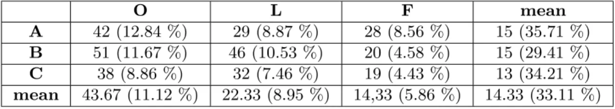
The texts were measured with LIX and OVIX. The results are shown in 4.1 and 4.2. The number of words that was replaced in all texts are shown i 3.1. The proportion of synonymous substitutions that were implemented and were of level 5 was in text A=66.67 %, in B=52.94 % and in text C=63.16 %.
Table 3.1: The table shows the number of synonym replacements, (and in parentheses the percentage), performed per text. O shows how many words that met the requirements to be replaced while the L and F show how many words that actually were replaced in each text. The percentage on ”same” is counted on all O words.
O L F mean
A 42 (12.84 %) 29 (8.87 %) 28 (8.56 %) 15 (35.71 %)
B 51 (11.67 %) 46 (10.53 %) 20 (4.58 %) 15 (29.41 %)
C 38 (8.86 %) 32 (7.46 %) 19 (4.43 %) 13 (34.21 %)
mean 43.67 (11.12 %) 22.33 (8.95 %) 14,33 (5.86 %) 14.33 (33.11 %)
The questions from the Scholastic Aptitude Tests were not used. They could have served as a check that participants did understand the text. But there was a risk that if the participants know that the text will be shown during the answering, they might not read as carefully as they should. The other way around, not having the text visible during answering would make it too difficult to answer the questions. Therefore, the questions were not included as they threatened to change the reading behavior.
3.3.3
Reading order
Reading three texts are quite demanding and it is also reasonable to assume that the participants are more focused in the beginning than at the end. Therefore it was important that all texts were present in all versions, in all different possible arrangements. So the three different texts in three different versions, but with the requirement that only one of the texts of the versions may occur at the same time
give 36 combinations. The texts were presented in the following order to the participants, see 3.2.
Table 3.2: The table shows the different combination in which the text were presented.
AO BL CF CO AF BL BL CF AO AF CL BO AO BF CL CO BF AL BL CO AF BF AL CO AO CF BL CO BL AF CL AO BF BF AO CL AO CL BF AL BO CF CL AF BO BF CO AL BO AL CF AL BF CO CL BF AO BF CL AO BO AF CL AL CF BO CL BL AF CF AL BO BO CF AL AL CO BF AF BL CO CF AO BL BO CL AF BL AO CF AF BO CL CF BO AL CO AL BF BL AF CO AF CO BL CF BL AO
3.4
Data Collection
When the participant came in to the room they were asked to sit down in front the eye-tracker. A paper was placed on the keyboard with a short instructional text that let them know that their eye movement would be recorded as well as the ethical guidelines of the study. When the participant was done reading the paper the table and chair were adjusted to optimize the eye movements recording. Then a calibration of the eye-tracker with four calibration points was performed. Holmqvist et al. (2011) writes that calibration is impor-tant for a variety of reasons. The eyeball radius between grown-ups varies by up to 10 % and may also have different shapes. He also writes that for maximal data quality, to always calibrate in the same
luminance conditions as during a data recording. These recommen-dations were followed, by having the same background colour when calibrating as the one that was behind the text. The colour was light grey.
The calibration was validated right after it was done and no result over 0.55 was accepted. If the value was over 0.55, the calibration was started over. This was done before every text to make sure that the data was of a good quality. The sampling frequency that was used was 500 Hz. This means that the eye-tracker records the gaze direction of the participants 500 times per second. This gives a pre-cision of 2 ms on the sampled data.
When the participant was finished reading a text, they pressed space-bar to move on to the next validation. Afterwards the participants were asked to fill in a form about their gender, age, native language and their email address in case they were interested in getting the results when the rapport was done.
3.5
Data analysis
The analysis for this study was divided into three parts: experiment 1, experiment 2 and experiment 3. In all experiments area of inter-est (AOI) have been used. AOI is a defined area on the stimuli that are especially of interest. In this case all original words that have a synonym candidate and all replaced synonyms had been made to AOI. This means that it is easy to access the data from these specific areas of the stimulus.
The data relevant for experiment 1 was fixation duration on AOI and on the whole text, number of fixations on AOI and on the whole
text and pupil size on AOI and on the whole text. The analysis that was done on all three measurements where AOI on one text compared with the other AOI on the other texts and the whole text compared with the other whole texts. Fixation duration and pupil size was also AOI on one text compared with the whole text to see if the AOI stood out from the rest of the text. This comparison could not be done on number of fixations because it is just a number that is relative to how many words the participant have read, while fixation duration and pupil size are the calculated averages.
The data relevant for experiment 2: extreme synonyms, were fixa-tion durafixa-tion and pupil size on extreme AOI, all AOI and the whole text. The analysis that was done on both measurements where the extreme AOI compared with the other extreme AOI. The extreme AOI were compared with the correlated all AOI and the extreme AOI were compared with the correlated whole text. By extreme means that all synonyms in the L text are at least four characters shorter than the original word and all synonyms in the F text occurs more than 100 times compared with the original word.
The reason why this was interesting is that it may not be worth it to replace all synonyms if the alternatives are just a little shorter or a little more frequent. Maybe the difference needs to be bigger in order to see a difference in the data. Also because every replaced synonym that is not controlled by a human has a risk of being a false synonym. False synonyms may have a negative impact on the read-ability level of the text. By only replacing the synonyms in extreme cases, maybe the risk of false synonym is weighed up by otherwise easily readable synonyms.
The data relevant for experiment 3: Synonym level 5, where fixa-tion durafixa-tion and pupil size on synonym level 5 AOI, all AOI and
the whole text. The analysis that was done on both measurements was the level 5 AOI compared with the other level 5 AOI. Level 5 AOI compared with the correlated all AOI, and the extreme AOI compared with the correlated whole text. Level 5 refers to the high-est level that people have ranked the synonym candidates in SynLex based on how good they think that the synonym candidate is in re-lation to the original word. The reason why this was interesting is because you want to avoid bad replacements. Maybe the synonym candidates on level 4 are not good enough. Maybe only the synonym candidates on level 5 are synonymous enough. By only replacing the synonyms with ones on level 5, the risk of false synonyms might be avoided.
The texts were also compared using the readability metrics LIX and OVIX. Here the whole texts were compared with each other. All comparisons were done with a paired-sample t-test in SPSS Statis-tics 22. The effect size was calculated with Pearson’s correlations coefficient, r.
Results
This chapter presents the results from this study. First the results from the readability metrics are presented. Then the results from the eye-tracking camera are presented. First the results from experiment 1 are shown where the original words and synonym candidates are used. In experiment 2 the extremely short or frequent synonym candidates AOI are used. Last is experiment 3 which looked at the texts where only level 5 synonym candidates are used. The data from one of the participants, on one of the text were corrupt. This resulted in that the comparisons needed to be repeated on different sample sizes, 35 and 36. This are also why there is blanks in the tables below.
4.1
Readability metrics
Here the results from the readability metrics are presented. The results from the readability metrics show how similar the texts are in terms of number of words, number of sentences, number of long words (LIX) as well as in terms of word variation (OVIX). The texts
were compared with each other as A, B, C and as O, L, F.
4.1.1
LIX
Here the results from LIX are presented. The data which the statical analysis was done on is seen in table 4.1.
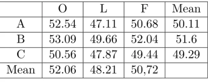
Table 4.1: LIX-value on all three versions of the three texts and respective mean value.
O L F Mean
A 52.54 47.11 50.68 50.11
B 53.09 49.66 52.04 51.6
C 50.56 47.87 49.44 49.29 Mean 52.06 48.21 50,72
O (M=52.06, SD=1.33) was significantly harder to read than L
(M=48.21, SD=1.31), (t(2)=4.7, p<.05, r=.96) and O was signif-icantly harder to read than F ( M=50.72, SD=1.3), (t(2)=5.18,
p<.05, r=.96). There was also a significant difference between L
and F (t(2)=-4.32, p=.05, r=.95).
There was no significant difference between A (M=50.11, SD=2.76) and B (M=51.6, SD=1.76), (t(2)=-2.56, p>.05, r=.88). Nor was there a significant difference betweenAandC(M=49.24,SD=1.35), (t(2)=1.05, p>.05, r=.6). But between B and C there was a signif-icant difference (t(2)=8.12, p<.05, r=.99).
4.1.2
OVIX
Here the results from the OVIX are presented. The data which the statical analysis was done on is seen in table 4.2.
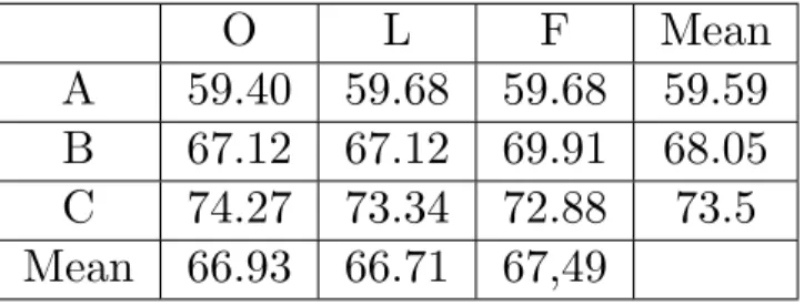
Table 4.2: OVIX-value on all three versions of all three texts and respective mean value.
O L F Mean
A 59.40 59.68 59.68 59.59 B 67.12 67.12 69.91 68.05
C 74.27 73.34 72.88 73.5
Mean 66.93 66.71 67,49
O (M=66.93, SD=7.44) was not significantly harder to read than L
(M=66.71, SD=6.84), (t(2)=.61, p>.05, r=.4) and O was not sig-nificantly harder to read than F ( M=67.49, SD=6.93), (t(2)=.69,
p>.05, r=.44). There was also no significant difference between L
and F (t(2)=.52, p>.05, r=.35).
There was a significant difference between A (M=59.59, SD=.16) and B (M=68.05, SD=1.61), (t(2)=-9.54, p<.05, r=.99). There was a significant difference between A and C (M=73.5, SD=.71), (t(2)=-27.93, p=.001, r=1). There was also a significant difference between B and C (t(2)=-4.3, p=.05, r=.95).
According to the LIX-value the texts A, B and C do not differ from each other (except B and C). According to the OVIX-value the texts do differ from each other but not by much. This, together with the fact that all three texts are represented in all three groups, ensures that the texts are similar enough.
When looking at the LIX-value it was discovered that O was sig-nificantly harder to read than both L andF.F was also significantly harder to read than L. When looking at the OVIX-value those dif-ferences were not seen.
4.2
Experiment 1
Here all original words and replaced synonym’s AOI were looked at. The measurements used were fixation duration, number of fixations and pupil size.
4.2.1
Fixation Duration
Here the results with fixation duration are shown. The data which the statical analysis was done on is seen in table 4.3.
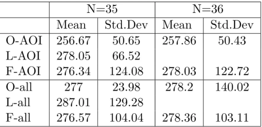
Table 4.3: The table shows the mean and standard deviation for the groups that have been compared.
N=35 N=36
Mean Std.Dev Mean Std.Dev
O-AOI 256.67 50.65 257.86 50.43 L-AOI 278.05 66.52 F-AOI 276.34 124.08 278.03 122.72 O-all 277 23.98 278.2 140.02 L-all 287.01 129.28 F-all 276.57 104.04 278.36 103.11
O-AOI has significantly shorter fixations thanL-AOI (t(34)=-2.14,
and F-AOI(t(35)=-.14, p=>.05, r=.14) nor is there significant dif-ference between L-AOI and F-AOI (t(34)=-.06, p=>.05, r=.01). When looking at the whole documents no significant difference be-tweenO-allandL-all(t(34)=-1.04,p=>.05, r=.18) is found. There is no significant difference between O-all and F-all (t(35)=-.02,
p=>.05, r=.00). Nor is there a significant difference between L-all and F-all (t(34)=1.66, p=>.05, r=.27).
There is no significant difference betweenO-AOIandO-all(t (35)=-.75, p=>.05, r=.13. Nor is there a significant difference between
L-AOI and L-all (t(34)=-.73, p=>.05, r=.12. This is also the case for F-AOI and F-all (t(35)=-.06, p=>.05, r=.01).
When looking at fixation duration, it can be seen that O-AOI has significantly shorter fixation duration than L-AOI.
4.2.2
Number of fixations
Here the results with number of fixations are shown. The data which the statical analysis was done on is seen in table 4.4.
O-AOI has significantly more fixations than L-AOI (t(34)=2.04,
p<.05, r=.33), but there is no significant difference betweenO-AOI
and F-AOI (t(35)=-.16, p=>.05, r=.03). There is, however, a sig-nificant difference between L-AOIandF-AOIshowing that L-AOI
has fewer fixations than F-AOI (t(34)=-2.66, p=<.05, r=.42). There is no significant difference between O-all and L-all (t (34)=-.31, p>.05, r=.05) and there was no significant difference between
O-all and F-all (t(35)=-1.1, p=>.05, r=.18). But there is a sig-nificant difference between L-all and F-all showing that L-all has
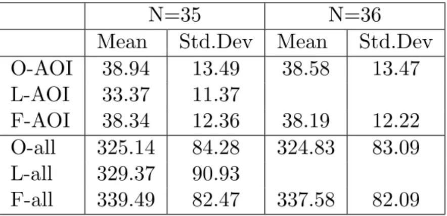
Table 4.4: The table shows the mean and standard deviation for the groups that have been compared.
N=35 N=36
Mean Std.Dev Mean Std.Dev
O-AOI 38.94 13.49 38.58 13.47 L-AOI 33.37 11.37 F-AOI 38.34 12.36 38.19 12.22 O-all 325.14 84.28 324.83 83.09 L-all 329.37 90.93 F-all 339.49 82.47 337.58 82.09
fewer fixations than F-all (t(34)=-.69, p=<.05, r=.12).
When looking at number of fixations could be seen that O-AOI
has significantly a greater number of fixations than L-AOI and that
F-AOI also has more fixations than L-AOI. Also, when looking at the whole document it was seen that L-all has fewer fixations than
F-all.
4.2.3
Pupil size
Here the results with the pupil size are shown. The data which the statical analysis was done on is seen in table 4.5.
There is no significant difference betweenO-AOIandL-AOI(t(34)=.82,
p>.05, r=.14) and there is no significant difference between O-AOI
and F-AOI (t(35)=-.06, p=>.05, r=.01). Similarly, there is no sig-nificant difference between L-AOI and F-AOI (t(34)=-.3, p=>.05,
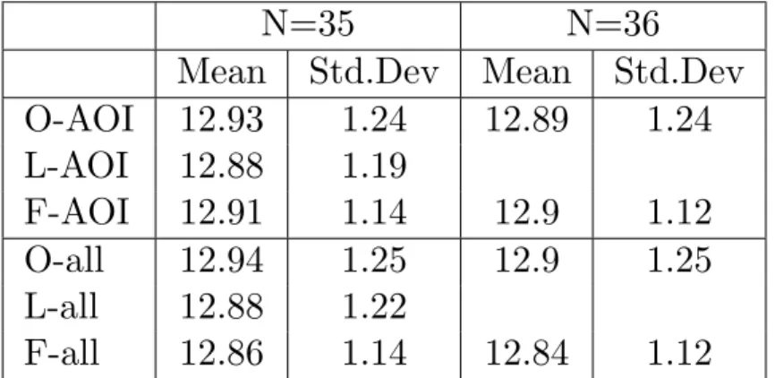
Table 4.5: The table shows the mean and standard deviation for the groups that have been compared.
N=35 N=36
Mean Std.Dev Mean Std.Dev
O-AOI 12.93 1.24 12.89 1.24 L-AOI 12.88 1.19 F-AOI 12.91 1.14 12.9 1.12 O-all 12.94 1.25 12.9 1.25 L-all 12.88 1.22 F-all 12.86 1.14 12.84 1.12
There is no significant difference betweenO-allandL-all(t(34)=.96,
p>.05, r=.16) and there is no significant difference between O-all
and F-all (t(35)=.69, p=>.05, r=.12). And there is not a signifi-cant difference betweenL-all andF-all (t(34)=.23,p=>.05, r=.04). There is no significant difference betweenO-AOIandO-all(t (35)=-.15, p=>.05, r=.03. Nor is there a significant difference between
L-AOI and L-all (t(34)=.35, p=>.05, r=.06. But there is a sig-nificant difference between F-AOI and F-all showing that the par-ticipants has bigger pupil size when reading F-AOI compared with
F-all (t(35)=3.54, p=<.001, r=.51.
When looking at pupil size it was seen that there was a significant difference between reading F-AOI and F-all showing that the pupil size was bigger when reading F-AOI.
4.3
Experiment 2: Extreme synonyms
Here the results from experiment 2 are presented. Extreme means that all synonyms in the L text are at least four characters shorter than the original word and all synonyms in the F text occurs more than 100 times compared with the original word. Here the extreme synonym pairs were looked at compared with the numbers from ex-periment 1, all replaced synonyms and the whole texts. In text A there were 6 synonym candidates that meet the requirement for L and 4 for F. In text B there were 13 synonym candidates that meet the requirement for L and 6 for F and in text C there were 4 synonym candidates that meet the requirement for L and 6 for F.
4.3.1
Fixation duration
Here the results with fixation duration are shown. The data which the statical analysis was done on is seen in table 4.6.
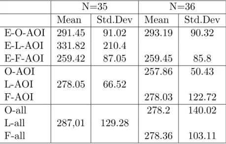
There is no significant difference between E-O-AOI and E-L-AOI
(t(34)=-1, p=>.05, r=.17). Nor is there a significant difference be-tween E-O-AOI and E-F-AOI (t(35)=1.76, p=>.05, r=.29). Nei-ther between E-L-AOI andE-F-AOI was there a significant differ-ence (t(34)=1.77, p=>.05, r=.29).
When comparing the results from the extreme AOI with the original AOI a significant difference is seen between E-O-AOI and O-AOI
showing that E-O-AOI resulted in longer fixation duration than O-AOI (t(35)=2.08, p=<.05, r=.34). Between E-L-AOI and L-AOI
there was no significant difference (t(34)=1.67, p=>.05, r=.27). Nor between E-F-AOI and F-AOI was there a significant difference (t(35)=-.68, p=>.05, r=.12).
Table 4.6: The table shows the mean and standard deviation for the groups that have been compared.
N=35 N=36
Mean Std.Dev Mean Std.Dev
E-O-AOI 291.45 91.02 293.19 90.32 E-L-AOI 331.82 210.4 E-F-AOI 259.42 87.05 259.45 85.8 O-AOI 257.86 50.43 L-AOI 278.05 66.52 F-AOI 278.03 122.72 O-all 278.2 140.02 L-all 287,01 129.28 F-all 278.36 103.11
When comparing the whole text with the extreme AOI no significant difference between E-O-AOI and O-allis seen (t(35)=.54, p=>.05,
r=.09). Between E-L-AOI and L-all there were no significant dif-ference (t(34)=1.21, p=>.05, r=.2). Nor between E-F-AOI and
F-all was there a significant difference (t(35)=-.77, p=>.05, r=.13). To summarize, there was a significantly difference between E-O-AOIandO-AOI showing that E-O-AOI resulted in longer fixation duration than O-AOI.
4.3.2
Pupil size
Here the results with pupil size are shown. The data which the stat-ical analysis was done on is seen in table 4.7.
Table 4.7: The table shows the mean and standard deviation for the groups that have been compared.
N=35 N=36
Mean Std.Dev Mean Std.Dev
E-O-AOI 12.9 1.27 12.86 1.27 E-L-AOI 12.93 1.16 E-F-AOI 12.93 1.19 12.93 1.18 O-AOI 12.89 1.24 L-AOI 12.88 1.19 F-AOI 12.9 1.12 O-all 12,89 1.25 L-all 12.87 1.24 F-all 12.84 1.12
There was no significant difference between E-O-AOI and E-L-AOI(t(34)=-.09, p=>.05, r=.02). Neither was there any significant difference between E-O-AOI and E-F-AOI (t(35)=-.25, p=>.05,
r=.04). Nor was there a significant difference between E-L-AOI
and E-F-AOI (t(34)=-.01, p=>.05, r=.00).
There were no significant difference between E-O-AOI and E-AOI
(t(35)=-.1, p=>.05, r=.02). Also, there was no significant differ-ence between E-L-AOI and L-AOI (t(34)=.19, p=>.05, r=.03). Nor was there a significant difference betweenE-F-AOI andF-AOI
(t(35)=.13, p=>.05, r=.02).
When comparing the extreme AOI with the whole document no sig-nificant difference between E-O-AOI and O-all was seen (t (35)=-.11, p=>.05, r=.02). Neither was there a significantly difference
between E-L-AOI and L-all (t(34)=.44 p=>.05, r=.08). No sig-nificant difference betweenE-F-AOI andF-all(t(35)=.33,p=>.05,
r=.06) could be found.
In summary, no significant differences at all could be detected.
4.4
Experiment 3: Synonym level 5
Here only the synonym candidates on level 5 were looked at. Level 5 refers to the highest level. People have ranked the synonym can-didates in SynLex based on how good they think that the synonym candidate are in relation to the original word. In text A there were 20 synonym candidates that meet the requirement for L and 17 for F. In text B there were 24 synonym candidates that meet the re-quirement for L and 10 for F and in text C there were 20 synonym candidates that meet the requirement for L and 13 for F.
4.4.1
Fixation duration
Here the results with fixation duration are shown. The data which the statical analysis was done on is seen in table 4.8.
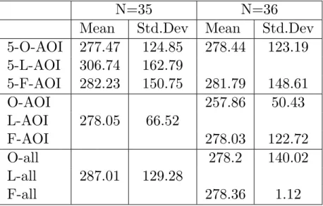
There was no significant difference between 5-O-AOI and5-L-AOI
(t(34)=-.84, p=>.05, r=.14). Neither was there any significant dif-ference between5-O-AOIand5-F-AOI(t(35)=-.1,p=>.05,r=.02). Nor were there a significant difference between 5-L-AOI and 5-F-AOI (t(34)=.65, p=>.05, r=.11).
There was no significant difference between 5-O-AOI and 5-AOI
(t(35)=.96, p=>.05, r=.16). Also, there was no significant differ-ence between 5-L-AOI and L-AOI (t(34)=1.08, p=>.05, r=.18). Nor was there a significant difference between 5-F-AOI andF-AOI
Table 4.8: The table shows the mean and standard deviations for the groups that have been compared.
N=35 N=36
Mean Std.Dev Mean Std.Dev
5-O-AOI 277.47 124.85 278.44 123.19 5-L-AOI 306.74 162.79 5-F-AOI 282.23 150.75 281.79 148.61 O-AOI 257.86 50.43 L-AOI 278.05 66.52 F-AOI 278.03 122.72 O-all 278.2 140.02 L-all 287.01 129.28 F-all 278.36 1.12 (t(35)=.12, p=>.05, r=.02).
When comparing the extreme AOI with the whole document no sig-nificant difference between 5-O-AOIandO-allwas seen (t(35)=.01,
p=>.05, r=.00). No significant difference could be found between
5-L-AOIandL-all(t(34)=.55p=>.05, r=.09). Nor was there a sig-nificant difference between 5-F-AOI and F-all(t(35)=.11, p=>.05,
r=.02).
In summary, there were no significant differences detected.
4.4.2
Pupil size
Here the results with pupil size are shown. The data which the statical analysis was done on is seen in table 4.9.
Table 4.9: The table shows the mean and standard deviation for the groups that have been compared.
N=35 N=36
Mean Std.Dev Mean Std.Dev
5-O-AOI 12.87 1.25 12.86 1.23 5-L-AOI 12.73 1.24 5-F-AOI 12,78 1.1 12.78 1.08 O-AOI 12.89 1.24 L-AOI 12.88 1.19 F-AOI 12.9 1.12 O-all 12.9 1.25 L-all 12.88 1.22 F-all 12.84 103.11
There is no significant difference between 5-O-AOI and 5-L-AOI
(t(34)=.47, p=>.05, r=.08). Nor is there a significant difference be-tween 5-O-AOI and 5-F-AOI (t(35)=.3, p=>.05, r=.05). Neither between 5-L-AOI and 5-F-AOI was there a significant difference (t(34)=-.19, p=>.05, r=.03).
When comparing 5-O-AOI and O-AOI, no significant difference is seen (t(35)=-.12, p=<.05, r=.02). Between 5-L-AOI and L-AOI
there was no significant difference (t(34)=-.56, p=>.05, r=.09). Nor between 5-F-AOI and F-AOI were there a significant difference (t(35)=-.43, p=>.05, r=.07).
When comparing the whole text with the AOI on level five no sig-nificant difference between 5-O-AOI and O-all is seen (t(35)=-.13,
p=>.05, r=.02). Between 5-L-AOI and L-all there was no signifi-cant difference (t(34)=-.54, p=>.05, r=.09). Nor between5-F-AOI
and F-all was there a significant difference (t(35)=-.23, p=>.05,
r=.04).
Analysis of results
This chapter discusses the results presented in chapter 4. First the analysis of results from the readability metrics will be discussed. Then the analysis from the eye-tracking camera with the measures of fixation duration, number of fixations and pupil size divided into experiment 1, experiment 2: Extreme synonyms and experiment 3: Synonym level 5 will be presented.
5.1
Readability metrics
According to LIX, the texts became significantly easier with both more frequent synonyms and shorter synonyms. Taking into consid-eration that LIX is very sensitive to word length, it is understand-able that the text with shorter synonyms got a lower LIX-value. The difference was bigger between the text with shorter synonyms than between the text with more frequent synonyms, this can also be ex-plained by LIX sensitivity to word length. In 33.11 % of the cases, the shortest word also was the most frequent, this explains why the text with more frequent words got a lower LIX-value then the
nal text.
The OVIX-value was not affected by either of the changes to shorter synonyms or to more frequent synonyms and the OVIX-values on the original texts varied much more than the LIX-values. This can be explained by the fact that OVIX takes into account the number of words as well as the number of unique words. When choosing the synonym candidate it was not noted if the that word already existed in the text or not, it was only noted if it was shorter or more fre-quent. If that had been taken into account, the OVIX-value would probably have been a little lower.
When looking at the different texts, no difference was seen between A, B and A, C according to the LIX-value. There was a significant difference between B and C but only on 2,31 and for LIX that is not a big difference. When looking at OVIX, there was a difference between all texts, because OVIX is sensitive to the number of words and number of unique words in a text. Text A, which got the lowest OVIX-value, was also shorter than the others by 100 words. There-fore it can be assumed that it is almost equal to text B and text C in number of unique words. Text B and C consisted of almost exactly the same number of words, therefore it can be assumed that text C has more unique words than text B. This together with the fact that the texts came from Scholastic Aptitude Tests gives the conclusion that the texts can be considered similar enough.
5.2
Experiment 1
Here the analysis of experiment 1 is presented. Experiment 1 in-cluded all synonyms that met the requirements for being replaced and the results of the whole texts. The measurements used were
fixation duration, number of fixations and pupil size.
5.2.1
Fixation duration
When looking at fixation duration, only one significant difference was seen between O-AOI and L-AOI, which showed that L-AOI gave sig-nificantly longer fixation durations than O-AOI. This goes against the hypothesis that shorter words will give shorter fixation durations. Even when looking at the other combinations, there was a small, but not significant, negative difference between the original texts and the ones with replaced synonyms. An explanation for this might be that because no consideration was put into choosing a synonym candidate that was semantically correct, some false synonyms could be found in the texts. When a synonym does not fit into the context, the reader could become confused, which could lead to longer fixations (Holmqvist et al., 2011).
When comparing the AOIs with the results from the whole texts, no significant differences were seen. But between the AOI and the whole texts there was a small non significant difference showing that the fixation durations were shorter in AOI compared to the whole texts. This may be explained by the fact that the words that are in the AOI are words that had a synonym candidate in SynLex. They are therefore words that someone wanted to be included in SynLex and words that have a synonym. It can therefore be assumed that they are fairly common words and therefore do not need as long of a fixation duration as other words that might not be as common.
5.2.2
Number of fixations
When measuring the number of fixations it was seen that L-AOI had fewer fixations than O-AOI. Between O-AOI and F-AOI there
were barely no differences at all. A reasonable explanation for why L-AOI had fewer fixations than O-AOI could be assumed to be that all the words measured in L-AOI are shorter than the original words and therefore demands fewer fixations to be perceived. According to Clifton et al. (2007), an AOI containing a long or unfamiliar word, receive more fixations than a short and familiar word. This effect is seen on L-AOI, which had fewer fixations than both O-AOI and F-AOI. The reason why the effect is not seen on F-AOI can be that the replacements that were done contained more false synonyms than L-AOI which disturbed the reading.
Loftus and Mackworth (1978) showed that significantly more fix-ations landed on semantically informative areas. A word that does not fit in to the context can be seen as a semantically informative area because it is a word that the reader does not expect to encounter and therefore could be confused by.
When looking at the whole document it was seen that O-all had fewer, but not significantly fewer, fixations than L-all and signifi-cantly fewer fixations than F-all. The reason for this is probably the same as the one for the AOIs. In L-all, which only had a few more fixations, it can be assumed that the false synonym AOIs may not have caused so many problems when the reader was looking at them, but later in the text they may have caused problems for the reader. It was probably the same thing that happened to F-all but to a greater extent.
5.2.3
Pupil size
When looking at pupil size it was seen that people had significantly bigger pupil size when reading F-AOI compared with F-all. This means that the words in F-AOI should be significantly harder than
the rest of the text. This also goes against the hypothesis that more frequent words would be easier to cognitively process. The same explanation as for the number of fixations can probably apply here. Too many false synonyms have replaced the original words in the F texts. Between O-AOI, O-all and L-AOI, L-all there was barely a difference at all which implies that the synonym candidates chosen here seem to be better than the ones chosen for the F texts.
When comparing O-AOI with L-AOI and F-AOI a small but non significant difference is seen and when comparing O-all with L-all and F-all also a small but non significant difference was seen. The reason that the difference was so small in the result can be due to that the results were counted on means and the differences may there-fore have been smoothed out. So just the fact that there are small differences could be taken seriously, they are just not significant.
5.3
Experiment 2: Extreme synonyms
Here the analysis of experiment 2 is presented. Experiment 2 in-cluded the synonyms that were extremely shorter or extremely more frequent, all synonyms that met the requirement of being replaced and the results of the whole texts. The measurements used were fixation duration and pupil size.
5.3.1
Fixation duration
The one comparison that was significant here was E-AOI and O-AOI showing that E-O-O-AOI resulted in longer fixation duration than O-AOI. Between E-L-AOI and L-AOI the same difference was seen but it was not significant. Between E-F-AOI and F-AOI the op-posite difference was observed. The explanation for this could be that a lot of the false synonyms among the more frequent synonyms
disappeared when only the extremely more frequent synonyms were used. The reason why the E-L-AOI got a little bit longer fixation duration than L-AOI could be because the fixation duration used was a calculated mean value. That means that if an average word gets two fixations with the first one being a longer fixation and the second one being a very short fixation, the mean value going to be low. But if the word is shorter it is probably only going to get one fixation and because the first fixation on a word tend to be longer than the rest (Holmqvist et al., 2011), the shorter word is going to get a longer fixation duration than the longer word. That is probably what happened here and for the rest of the compared data.
5.3.2
Pupil size
In this comparison, no difference was significant. This is probably because of the same reason as the first comparison done with pupil size. The differences that may have been there have evened out when the mean was calculated. But when looking at table 4.7, small differences are seen. E-L-AOI and E-F-AOI gave a little bit bigger pupil size than E-O-AOI, which indicates that E-L-AOI and E-F-AOI should be a little bit harder to read than E-O-AOI. When looking at E-O-AOI it is seen that it gave a smaller pupil size then both O-AOI and O-all, which is indicating that the words in the AOI should be easier to read. Both E-L-AOI and E-F-AOI got bigger pupil sizes than L-AOI and L-all respective F-AOI and F-all. This indicates that the chosen words are harder to read than the rest of the text even though they are extremely short or extremely more frequent.
5.4
Experiment 3: Synonym level 5
Here the analysis of experiment 3 is presented. Experiment 3 in-cluded the synonyms that were on level 5, all synonyms that met
the requirement of being replaced and the results of the whole texts. The measurements used were fixation duration and pupil size.
5.4.1
Fixation duration
Here, there were no significant differences but 5-O-AOI, 5-L-AOI and 5-F-AOI got longer fixation durations than O-AOI, L-AOI and F-AOI. An explanation for this could be that in some cases there seemed to be particular word which participants got stuck on. That resulted in some fixation durations being over 15 000 ms, compared with a normal fixation on 200-300 ms, which is quite a long time. When the mean was calculated on all fixations on each text or on all AOIs in a text, that was evened out. Now when the values are based on such few words, a value like 15 000 ms is quite devastating for the results. The same explanation goes for 5-O-AOI, 5-L-AOI and 5-F-AOI compared with O-all, L-all and F-all.
When comparing 5-O-AOI, 5-L-AOI and 5-F-AOI no significant dif-ference is seen. 5-L-AOI got a slightly longer fixation duration than 5-O-AOI and 5-F-AOI and that can probably be explained by the same theory as the results in experiment 2. Because the words are shorter in 5-L-AOI than the other groups, it probably had fewer but longer fixations. Holmqvist et al. (2011) writes that if the trial time is constant, it will be a inverse relationship between number of fixa-tions and fixation duration. The trial time was not controlled here but it is probably what happened here.
5.4.2
Pupil size
In this comparison, no difference was significant. This is probably also because of the same reason as the first comparison done with pupil size. The differences that may have been there have been
evened out when the mean was calculated. But looking at the table 4.9, small differences are seen. For all cases the AOI with only level 5 synonyms had a smaller average pupil size than the original AOI. That can be interpreted as the synonyms on level 5 being easier to read than the original AOI. And in all cases the synonyms on level 5 had a smaller average pupil size than the whole texts, which also can be interpreted as the more extreme ones being easier to read than the rest of the texts.
Discussion
This chapter begins with a discussion about the procedure and lim-itations of this study and then the results are discussed.
6.1
Procedure
The fact that a within-group design was chosen was to the study’s advantage. Because reading style is very personal and for example pupil size can vary quite a lot from person to person, it was good that all participants could be represented in all conditions. The reason that this was possible without having to worry about the participants experience a learning effect was that the conditions were presented in three different texts.
The texts were quit similar according to the readability metrics. The differences that existed were evened out by the fact that all partici-pant had to read all of them, in a different order. Because all texts were read the same number of times and the different text occurred the same number of times in all different conditions, the difference
between the texts becomes negligible. One disadvantage with eye-tracking is that the texts that were used had to be short enough to fit on one computer screen to avoid the participants having to use the scrollbar and thereby avoid creating an unnatural reading pattern. When it comes to the participants, all of them were students at Link¨opings University. That is a quit narrow sample but the bene-fits of selecting students for this type of task is that they probably have similar reading habits and that the text was not to hard for them to read. This is also a disadvantage because the generalizabil-ity is reduced. No questions were asked regarding dyslexia or other similar reading problems, which increases the generalizability.
The synonym candidates were chosen by searching for synonyms in SynLex. An advantage with this is that it is simple and that SynLex is quite big with 80 000 synonym pairs. A disadvantage is that no consideration was put in to the context the word came from when the synonym candidates were chosen. That means that it might have been better synonyms on level 4, but because there were suggestions on level 5, the synonyms on level 4 were not taken in to consideration.
6.2
Results
Almost no difference became significant during the comparison. That means that the few small differences that showed, probably just are random. However they may be seen as trends.
The reason that some differences became significant can be due to that a large number of statistical tests have been performed, which can lead to type 1 error. Type 1 error means that a significant dif-ference is found, when in fact there is none. There is a risk that the
found significant differences are just type 1 errors. The opposite can also have occurred. The opposite is type 2 error which means that there is a difference but it is not found. Type 2 error can occur when the tested sample is to small or the sample do not have a normal distribution. In this case a type 2 error almost could be excluded because sampling distribution tend to be normal regardless of the population distribution in samples of 30 or more and the used sam-ple consists of 36.
In an attempt to see a difference between the replacement strate-gies the number of times each strategy got a result that was lower than the results of the original text, were counted. In this compar-ison a difference was seen. Always choosing a shorter word resulted in a lower value (regardless of measurement) than the original text 3 of 8 times. Always choosing a more frequent word resulted in a lower value compared with the original text (regardless of measurement) 2 of 8 times. According to this it should be a little bit better to choose a shorter synonym. But the differences were quite big between the texts with shorter synonyms. In 4 of 8 times were the difference be-tween the results from the text with more frequent synonyms almost non-existent. Based on this, neither a shorter synonym or a more frequent word can be recommended.
When only looking at the results from experiment 2: extreme syn-onym, a difference was seen. With these settings, always choosing a extremely shorter word resulted in a lower value (regardless of used measurement) than the original text 0 times. Always choosing a ex-tremely more frequent word resulted in a lower value compared to the original text (regardless of used measurement) 3 of 6 times. Also according to this results, it should be a little bit better to choose a more frequent word.
When only looking at the results from experiment 3: synonym level 5, no difference was seen. With these settings, always choosing a shorter word, but with a synonym level of 5, resulted in a lower value (regardless of used measurement) than the original text 3 of 6 times. Always choosing a more frequent word, but with a synonym level of 5, resulted in a lower value compared with the original text (regardless of used measurement) 3 of 6 times. According to this results, while the synonym level are 5, it does not matter if the syn-onym is more frequent or shorter then the original word.