Stochastic gradient optimization of importance sampling for the efficient simulation of digital communications systems

Stochastic Gradient

Optimization of Importance

Sampling for the Efficient

Simulation of Digital

Communications Systems

w.

A.

Al-Qaq

M. Devetsikiotis

J.

K. Townsend

Center for Communications and Signal Processing

Department of Electrical and Computer Engineering

-North Carolina State University

Submitted to the IEEE Transactions on Communications

Stochastic Gradient Optimization of Importance Sampling for the

Efficient Simulation of Digital Communication Systems

1

Wael A. AI-Q a q2 Michael Devetsikiotis

J. Keith Townsend

Center for Communications and Signal Processing, Department of Electrical & Computer Engineering, North Carolina State University, Raleigh, NC 27695-7914

Tel: (919)515-5200 Fax: (919)515-5523

Abstract

Importance sampling (IS) techniques offer the potential for large speed-up factors for bit error rate (BER) estimation using Monte Carlo (MC) simulation. To obtain these speed-up factors, the IS parameters specifying the simulation probability density function (pdf) must be carefully chosen. With the increased complexity in communication systems, analytical optimization of IS parameters can be virtually impossible.

In this paper, we present a new IS optimization algorithm based on stochastic gradient techniques. The formulation of the stochastic gradient descent (SGD) algorithm presented in this paper is quite general and system-independent, and its applicability is not restricted to a specific pdf or biasing scheme. The generality and effectiveness of the SGD algorithm are demonstrated by two examples of communication systems where IS techniques have not been applied before. The first example is a communication system with diversity combining, slow nonselective Rayleigh fading channel and non coherent envelope detection. The second example is a binary baseband communication system with a static linear channel and a recursive least square (RLS) linear equalizer in the presence of additive white Gaussian noise (AWGN).

IPortions of this work were presented at GLOBECOM '93.

Stochastic Gradient Optimization ... , Al-Qaq, Devetsikiotis, and Townsend

1

Introduction

1

Importance sampling (IS) techniques can substantially accelerate bit error rate (BER) es-timation using Monte Carlo (MC) simulation, provided that the proper IS biasing scheme and parameter values are used. Analytical optimization techniques [1, 2] typically require a closed form expression for the IS estimator variance. Optimization of IS parameters us-ing techniques based on large deviations theory (LDT) are applicable to a larger class of problems, including systems with additive Gaussian noise and a "moderate nonlinearity"

[3, 4, 5].

Efficient simulation methods of communication links characterized by slow, time varYIng channels and linear least mean square adaptive equalizers were recently presented in [6].

Approaches that optimize IS parameters based on statistical estimates of the IS estimator variance are more system independent [7, 8]. The most general of these techniques uses mean field annealing (MFA), a stochastic optimization algorithm, to perform the optimization [8]. However, the MFA approach can be affected by long run times due to high dimensionality in the IS parameter space.

In this paper, we formulate and develop an IS methodology for the efficient simulation of low BER digital communication systems based on stochastic gradient descent (SGD) optimization. In this methodology, near-optimization with respect to the IS parameters is achieved by using a SGD in the cost function (IS estimator variance). Furthermore, this methodology is combined with an IS methodology derived in [4] using a conditional IS scheme to further improve the IS estimator efficiency. In [9], we present the SGD approach in the different context of queueing system simulation.

Stochastic Gradient Optimization ... , Al-Qaq, Devetsikiotis, and Townsend ₂

We demonstrate the effectiveness of the SGD algorithm via two practical examples where

IS techniques have not been applied before. The first example is a communication system in

a frequency nonselective Rayleigh fading channel with diversity and noncoherent envelope

detection of binary orthogonal FSK signaling [10]. In this example, the SGD algorithm is used to determine the optimal nonuniform variance scaling (VS)parameters of Rayleigh

dis-tributed random variables. The second example is a binary baseband communication system with a static linear channel and an RLS linear equalizer in the presence of additive white

Gaussian noise (AWGN). Here, the SGDalgorithm is applied to search for the near-optimal

IS parameters in a 3D-dimensional space using mean translation (MT) [2] and nonuniform

VS (11] as a biasing technique.

The conditional IS formulation and the SGD algorithm are introduced in Section 2and 3

respectively. The examples as well as the simulation results are presented in Section 4. Our

results show runtime speed-up factors of 2 to 10orders of magnitude for second and fourth order diversity systems with noncoherent envelope detection. Speed-up factors include the

overhead of the SGD algorithm. Speed-up factors of 6 to 9 orders of magnitude were also obtained for the RLS adaptive equalization example for error probabilities in the range of

10-6 _{to 10-}9_•

2

Conditional Importance Sampling Formulation

Consider a communication system with two input random vectors X and Y. The random

vector X is assumed to be m-dimensional with a marginal probability density function (pdf)

!x(X,

8), where 0 is a parameter vector. The conditional pdf of the n-dimensional random vector Y given X is assumed to be Gaussian with a mean vectorJ.L and a diagonal covariance

matrix :EYIX = ~In, where L, is an n X n identity matrix. This conditional pdf will be denoted as !YIX(Y,JLIX). Let the decision random variable G(X, Y) (G : ~m X ~n ~ ~)

be a nonlinear transformation of the random pair (X, Y) to the decision space, and let

Stochastic Gradient Optimization ... , Al-Qaq, Devetsikiotis, and Townsend

The probability of a detection error P is given by

3

J

{k(x)

!YIX(Y,

JLIX)dY}

!x(X,

8)dX

Ee{EJJ{lo(X)}}

Ee{P(X)} (1)

(2)

(3)

where

P :

iRd(0 )

x

iRn -+

[0, 1] ,

and d(8) is equal to the dimensionality of the parameter vector 8. Ee { .} and EJ.l{.} denote the expectations with respect to the pdf's !x(X,0)

and !YIX(Y,

JL!..tY)

respectively. lo(X) is the indicator function of the set !l(X)

==

{Y :

I(G(X,

Y))

=

I} (lo(x)

=

1 when Y E f2(X) and lo(x)

=

0 when Y FJ. !l(X)), and

P(X)

is

the conditional probability of a detection error given the random vector X. A

Me

estimator of (1) is given by the sample mean expression

1 N.x:

P

=

N

I:

p(X(j))

X i=l

with

F(X(j))

=

~ ~

I(G(X(j),Y(i,j)))

y i=l

where X(j) and Y(i,j) are i.i.d. repetitions of X and Y, respectively. In order to apply IS, observe that (1) can be written as

P

=

P(0,JL)

=

J

{k(X)WYIX(Y'JL'JL~IX)fYIX(Y'JL~IX)dY}WX(X,8,8*)fx(X,8*)dX

_ Ea -{EJl~

{l

o(X)wYIX(Y,JL,JL~IX)}wx(X, 8, 8*)}

_ Ee-{P(X)wx(X,8, 8*)}

(4)

where the IS weight functions are given by

and

wx(X,

8, 0*)

=

!x(X, 0)/!x(X, 0*)

(5)

(6)

Stochastic Gradient Optimization... , Al-Qaq, Devetsikiotis, and Townsend ₄

1, · · ·

,Ni

are drawn from a marginal biased density!x(X,

e*).

For each fixed

i,

independent samples Y(i,j), i = 1. .. ,

Ny,

are drawn from a biased conditional density !YIX(Y,JL;IX).

Thus, we have the following IS estimator 1 Ni:

P

=

N* L P(X(j))wx(X(j),

e, e*)

X j=l

where the conditional IS estimator P(X(j)) is given by

A 1

Ny

P(X(j))

=

N* LI(G(X(j), Y(i,j)))wYIX(Y(i,j),JL,JL;IX(j))

y i=l

(7)

(8)

It is easy to show that the estimator in (7) is an unbiased estimator of P. It was shown in [4] that the variance of (7)is given by

V{P}

V(0,0*,JL,JL;)

(VI

+

Ny V2)/(NiNy)

(9)

where V :lRd(0 ) x lRd(00) x ~n X lRn ---+

[0,

00),

and

V2

=

Ve-{P(X)wx(X,0, 0*)}

(10)

(11)

Ve- {.} and Vu: {.}_.., denote the variances with respect to the simulation pdf's. The empirical precision of the estimator in

(7)

may be found by using the sample variance estimator

fi· A

1 x

p2

V{p}

=

N*2 L P2(X(j))wi:(X(j),

e,

e*) -

N*

X ;=1 X

(12)

For a given relative precision ao

>

0, the simulation is terminated when the condition

';V{P}/

P :::;

eto is satisfied.

Stochastic Gradient Optimization ... , Al-Qaq, Devetsikiotis, and Townsend ₅

parameter vectors J.L~t and 8~t. In the examples considered in this paper, the components of X are dominant. Thus, choice of the marginal simulation distribution !x(X, e*) will

significantly impact V {P} and the efficiency of the applied IS methodology. Selecting an optimal !x(J'Y,0*) is typically a difficult task since it involves a joint minimization of

Vi

and

Vi·

In this paper, optimization of !x(X,0) is achieved using a stochastic gradient descent (SGD) algorithm which is described in Section 3. Optimizing the conditional simulation distribution !YIX(Y,

JL;

IX) for every X

==

X, will in effect minimize the conditional variance

(;y)V~;{ln(x)wYIX(Y,J.L,J.L~IX)}. The approach we adopt to minimize this conditional variance is given in

[4]

and summarized in the next subsection.

2.1

Minimization of the Conditional Variance

In this Section, we summarize the method of mean translation (MT), as discussed in [4], in order to minimize the conditional variance

Vi

in (10) for every given X. Let af2(X) de-note the boundary of the set n(X). Consider a conditional simulation density of the form

fYlx(Y,J.L~IJ'Y)==

(2:)n/2

ex p

(- , II

Y - J.L~1I2/2). It was shown in

[4]

that for the conditional simulation density to be asymptotically optimal, two conditions must be satisfied: the con-dition liID.-r-+ooJ.L; = J.L~ = J.L~t, and the forbidden set condition. J.L~t E af2(X) is called a minimum rate point. For the examples considered in this paper, there is always a unique minimum rate point. The case where there are multiple minimum rate points is discussed in

[3].

The asymptotically optimal !YIX(Y,JL;IX) is given by

(13)

Thus, the problem of determining the asymptotically optimal conditional simulation distri-bution

hIX(Y,

JL~tIX)reduces to identifying the minimum rate point JL~t· Determining

JL:"t

Stochastic Gradient Optimization ... , Al-Qaq, Devetsikiotis, and Townsend

subject to

6

(14)

Later on, the set an(..IY) will be defined in the context of the examples considered in this paper. In the subsequent notation, the parameter vector JL; will be replaced by JL':.r,t.

3

The Stochastic Gradient Descent (SGD) Algorithm

After choosing !YIX(Y,J.L~tl..lY), our next goal is to determine the marginal simulation dis-tribution !x(..IY,8*) in order to minimize V

{P}

in (9), which for most practical cases does not have a closed form expression. It was justifiably argued in [4] that for the op-timal !YIX

(Y,

J.L~t

1..1\)

derived in the preceding Section, V{p} is minimized by selecting

fx(~Y, e~t) ex:

P(..IY)!x(X,0).

The difficulty encountered with this simulation pdf is that in most practical cases its implementation leads to a tautology because it requires knowledge of the probability of error Pin a closed form. In

[4,5],

approximations based on ideal cases were made to yield implement able but suboptimal marginal simulation pdf's.

This difficulty is surmounted by using an algorithm based on a stochastic gradient tech-nique to specify the near-optimal IS parameter vector that will minimize the cost function

V{P}

in (9). To begin, let the gradient of

V{F}

=

V(e,e*,JL,JL':.r,t) with respect to 0* be denoted as

vre.V{F}

==

V'0.V(0,0*,JL,JL~t). It is well known

[12],

that

(15)

constitutes a necessary, but not a sufficient, condition for a vector 0~t to be a local or global minimum of V(0,e*,p"JL~t). Thus, in seeking a minimum, the optimization algorithm involves a descent in the cost function V{p}

=

V(0,0*,/.L,J.L':.r,t) in a direction given by V"e.V(0, O",JL, p,':.r,t). This well known deterministic gradient descent (DGD) algorithm [12], is an iterative scheme with the kth iteration given by

(16)

Stochastic Gradient Optimization ... , Al-Qaq, Devetsikiotis, and Townsend ₇

Since in most practical applications, a closed form expression of Ve.V(0,E).,JL,JL~t) is not available, we use an unbiasedestimate

V

e.V(E), E).,JL,JL~t) of the gradient. Replacing the deterministic gradient with its unbiased stochastic estimate results in the following stochastic gradient descent (SGD) algorithm

(17)

The algorithm in (17) is of the Robbins-Monro (RM) type [13, 14]. In this paper, this algorithm is used to specify the near-optimal IS parameters, namely 8~t. The almost sure convergence (i.e., Prob{limJc--.oo e*(k) = e~t}

=

1)of an RM type algorithm like the one in (17) is proved in [14] provided that a proper step size

j3(

k) is chosen. The RM algorithm is used in a variety of applications such as least mean square adaptive filtering (the Widrow algorithm)

[15]

and stochastic steady-state optimization of regenerative systems

[16].

In order to apply the algorithm in (17), we need to derive an expression for an unbiased estimate ofV'a-V(0, O",JL,JL~t) using an approach (similar to [13, 17]) based on the following proposition:

Proposition 1 Let 0 ::; I(X)

<

00 be independent ofthe parameter vector 8* with

Ea{I(X)wx(X, 0,e*)}

<

00, and let wx(X,8,0*) be continuously differentiable with

re-spect to

0*.

Then we have

V'a-Ea-{l(X)wi(X, 0, 8*)} yre-Ee{I(X)wx(X,8,e*)}

Ee{l(X)V' e-wx(X,

0,0*)}

Ee-{I(X)wx(X,

8, 0*)\7 e-wx(X, 0, 8*)}

(18)

(19)

Proving the above proposition merely requires the justification of interchanging the gradient and expectation operators in (18). This is done in the Appendix. Note that the last step in (19) is simply a result of applying the IS weight function wx(X,E),0·) to (18). This step will prove to be valuable in implementing the SGD algorithm.

Stochastic Gradient Optimization ..., Al-Qaq, Devetsikiotis, and Townsend

where

8

(20)

and

We can estimate (20) using the following unbiasedestimator

(22)

Note that the result in

(23)

can be attained by simply taking the gradient of the first term on the right-hand side of

(12),

interchanging the gradient and summation operators, and multiplying the result by 1/2.

Observe that during the course of performing the SGD algorithm in (17), the IS weight function wYlx(Y,JL,JL~tIX)wx(X,8,8·(k))is used in the IS estimator of all three quanti-ties, namely P, V{p}, and V'0-V{p}. Although in the limit as k ~ 00 this approach yields

an optimal distribution function !x(JY,0~t) for the estimator of P, it will generally provide suboptimal estimates of V{p} and V7o-V{p}. Fortunately, in most practical cases these suboptimal estimates are sufficiently accurate to successfully perform the SGD algorithm. The ability to use the IS pdf !x(JY,0*(k)) at the kth iteration in all three estimates is very valuable in implementing the simulation algorithm efficiently, because it permits the SGD algorithm to be started at a point,

8*(1),

where there is a sufficient "raw" (i.e., unweighted) error count to accurately estimate

(20)

using

(23).

Also, the fact that the optimal condi-tional simulation distribution !YIX(Y,JL~tIX)is used in

(23)

contributes to a better estimate of (20).

3.1

The SGD

Simulation

Algor'it hm

For a given signal to noise ratio (SNR) and a fixed relative precision ao

>

0, the algorithm

Stochastic Gradient Optimization... , Al-Qaq, Devetsiliotis, and Townsend

• For k

=

1, 2, ...

For j = 1,2, ... ,N_JT

*

Sample

X(j)

from

!x(X,

e*(k))

*

Compute

wx(X(j),

e, e*(k)) using (6) and

\leowx(X(j),

e, e*)leo=eo(le)

*

Compute J.L~t,j by solving

(14)

*

For i

=

1, ... ,

Ny

· Using J1.~t,j' sample

Y(i)

from fylx(Y,J1.~t,jIX(j))

· If an error is detected, compute wYIX(Y(i),J1.,J1.~t,jIX(j))using (5)

· Next i

*

Compute p(X(j)) using

(8)

*

Next j

Compute

P

using (7),

V

{F}

using (12), and

\leo

V

{F}leo=eo(le)

using (23)

- if

a(k)

=

jV{P}/ F

~

a

o stop, else

Compute

e*(k

+

1)

using

(17)

Next k

9

To overcome the difficulty involved in specifying a starting point e*(l), the above

algo-rithm can be applied at a low SNR

(F

= 10-2

"-J 10-3) . Thus, 0*(1)

=

0 (or some starting

point in the proximity of e) can be used to accurately estimate VeoV{F}leo=eO(l) using a

reasonable number of decisions

(Ni

x

Ny

=

100 "-J 1000). The optimal parameter vector

e:"t

determined for a low SNR is then used as the starting point 0·(1) at a higher SNR

and so on. With this technique applied efficiently, the overhead Noh (in number of decisions)

involved in determining 0:"t at a high SNR willbe insignificant compared to the savings in

number of decisions

Ni

x Ny needed to accurately estimate a low P. In other words, for a given accuracy we would still have

Nx

x Ny ~

Ni

x

Ny

+

Noh.

In the examples considered in this paper, a fixed step size {3 was used in (17). The

Stochastic Gradient Optimization ... , Al-Qaq, Devetsikiotis, and Townsend ₁₀

To Decision Device

Figure 1: Model of a digital communication system with diversity reception.

terminated, namely a(k) :::; 0:_{0 •} For a given application, a fixed step size

f3

is experimentally

chosen to assure a convergent behavior of the SGD algorithm. As in the case of the DGD

algorithm, it was observed that for small values of j3 in

(17),

the sequence {E>*(k)} would closely follow the correct path of the gradient descent. However, the use of very small step

sizes would result in a very slow convergence rate. On the other hand, the use of larger

step sizes increases the rate of convergence, but may cause a deviation from the correct path

of the gradient descent. Therefore, choosing {3 is a design issue based on trade-off between accuracy and overhead.

4

Applications and Simulation Results

4.1

Diversity Reception in a Nonselective Rayleigh Fading

Chan-nel

Fig. 1 shows the block diagram of a digital communication system in which Lth order di-versity reception is used to compensate for the distortion caused by a non-selective fading channel and additive noise. A frequency non-selective channel results in a multiplicative

Stochastic Gradient Optimization ... , Al-Qaq, Devetsikiotis, and Townsend ₁₁

process may be regarded as a constant for the duration of at least one signaling interval [10].

Thus, if the transmitted signal is u(t), then the received equivalent complex lowpass signal on the ith diversity over one signaling interval (0 ~ t ~ T) is given by

i

==

1, ...,L

where for all i, 1 :::; i :::; L, c; is the fading gain of the ith fading channel which is a complex

Gaussian random variable (CGRV) with E{Ci} == 0 and

E{ICiI

2_}

₌₌

_2u2

• The complex

additive noise on the ith antenna is given by Yi(t), where each Yi(t) is a complex AWGN with E{Yi(

t)}

==

0and E{Yi(t)Yi*(t

+

T)}

=

2YQ5(

r)

(* denotes the complex conjugate), with Yi(t) and Yj(t) being independent processes for i

=I

j.

For noncoherent detection, we consider envelope detection

[10]

with binary orthogonal FSK signaling. In this case, the optimum demodulator for the signal received from the ith

diversity consists of two matched filters, with impulse responses Ul(t - T) and U2(t - T)

respectively, where

Ul(t)

=

It;

exp(j27rtljt) , and

U2(t)

=

~exp(j47rtljt). In the case of orthogonal signaling, the quantity p

==

~

J

Pl(t)P2(t)dt is zero. Let the sequences {Xli} and {X2i} be i.i.d. Rayleigh random variables (RRV's), with

E{xi

_{i }}

==

20"2 and

E{x;i}

==

2YQe,

and let the sequences{v«} and

{Y2i}

be i.i.d. zero-mean Gaussian random variables (GRV's), with E{Y~i}

==

E{Y~i}

=

YQe. Then if welet

and

the decision variable for noncoherent envelope detection will be given by

L

G(X, Y)

==

L

g(Xli' X2i, Yli, Y2i)

i=l

where for i

=

1, ...

,L

(24)

Stochastic Gradient Optimization ... , Al-Qaq, Devetsikiotis, and Townsend ₁₂

It is important to point out that in most practical communication systems with Rayleigh fading channels, the Rayleigh fading process X is more dominant compared to the AWGN process Y. Hence, choice of the marginal simulation distribution fx(~Y,e*) will significantly impact V{p} and the efficiency of the applied IS methodology.

Note that Y is an n-dimensional (n == 2L) zero mean Gaussian random vector with a conditional diagonal covariance matrix :Ey\X

=

~r,., (-y

=

1/1'0£).

We apply the result in (14) to minimize the conditional variance

Vi

in (10) for every given X. In this case

8f2(X)

==

{Y : G(X, Y) = O}. Thus, we need to minimize IIYl12 subject to G(X, Y) =

o.

Solving this constrained minimization using the Lagrange multipliers technique [12], yields

* [ . * •

*]

h f-Lopt

==

J.Lll'J-L21' • • • ,f-LlL ,J.L1L were

1 L

J.L~i

== - -

L

eXli - X2i

L i=l

i = 1, ...,L

and J-L;i

==

0,i

==

1, ...,L.

After choosing !Y1X(Y,/-L~tIX), we turn our attention to choosing the optimal marginal simulation distribution !x(X, e~t)in order to minimize (9). For an Lth order diversity sys-tem, observe that the decision variable in

(24)

is the sum of the i.i.d. r.v.'sg(Xli' X2i, Y1i, Y2i). As a result, it can be easily shown that since the random variables {Yi} are equally biased, the random variables {Xi}, i == 1, ... ,L should be equally biased as well. This reduces a 2L-dimensional search in the space of

e*

to a two-dimensional search. Thus, if we let

0*

==

[0-;,

0";]t

("t"

denotes the transpose), this will result in the following simulation distri-bution

with the gradient of the IS weight function given by

... ... * _

[8

WX(X ,0,0*) owx(X,0,

e*)]

t

'\J

e.wx(X, 0, 0 ) -

a •

1

8 •

0"1 0"2

where

8wx(X,_{0, e*)}

[2L

_2:f:l

_Xli]

_{(X 0 0*)}

--~---==

- -

w x " ,

8_0",~ (j~J (j~3J

Stochastic Gradient Optimization ... , Al-Qaq, Devetsikiotis, and Townsend ₁₃

Define the SNR per diversity as Eb/No

=

~E{xiJ/2YQe. For a given SNR per diversity and a fixed Q o

>

0, the SGD algorithm starts with a first order diversity and progresses to

higher order diversities. Since an increase in diversity order corresponds to an increase in the

effective SNR, we can apply the technique discussed in the previous section. Specifically, we

simulate a second order diversity system using the same procedure, with the starting point

being 8~t of a first order diversity system. This approach willeffectively place the starting point in a neighborhood close to the optimal, thereby contributing to a better estimate

of \7e-V

{F}

and reducing the number of iterations required to locate the near-optimal IS

parameters.

For example, the starting point 8* for a second order diversity system at a SNR of 20

dB was chosen as 0~t ~ [.0716, .0725] of a first order diversity system at the same SNR

(F

=

2.5 X 10-a,

e

=

[.707, .05]). To attain e~t for a first order diversity, only N.

r

x Ny

=

100 x 1 decisions were used in (7) and (23) to estimate P and yr0-V

{F},

respectively, at each iteration. It was empirically observed that the variance of V'0-V

{F}le-=e-(k)

improves

as k increases (i.e., as the minimum is approached). The simulation was terminated when

a(

k) became less than Uo

=

.15 based on 100 decisions. In general, the SGD algorithm

may be used to simulate an Lth order diversity system with the starting point being the

optimal simulation density of a diversity system of order L - 1 or L - 2. A fixed step size of

j3 ::;

10-

2_min{O";

_(1),

_O"i

_{(I)} /}

_II

_V'

_0-

_V{F}

_10-=0-(1)

_II,

_{was experimentally observed to guarantee}

the convergence of the SGD algorithm.

The results of applying the above algorithm to second and fourth order diversity systems

along with the optimal IS parameters are shown in Table1for a per-diversity SNR of 20 and 30 dB . Note that since the asymptotically optimal translation JL~t is determined in closed

form, rather than numerically as in [4], the cost of sampling Y is insignificant. Therefore,

we chose

Ny

==

1 for the simulations. This choice of

Ny

is justified by recalling that, for most practical cases, Y is not the main contributor of randomness in the communication

system being considered. In each case, the transmit filter was normalized

(e

=

1).

V{p}

was calculated using an ensemble of NE

==

20 estimates of P. Note that for a given SNR,

Stochastic Gradient Optimization ... , Al-Qaq, Devetsilciotis, and Townsend

(E&/No ) L 0·o-pt

P

V·{P}

Speed-up(Sp) NXxN

y

Noh

20 dB 2 .0802 7.9825 x 10-5 _4.7x10-1 1 _3.92

XlQ2 1000X1 63.1X1Q3 .0705

20 dB 4 .0844 2.5928X10 8 9.48X10-18 6X105 1000X1 67.1X1Q3 .0686

30 dB 2 .0253 8.1684x 10-7 _{3.3 X10- 15 4.07X1Q4 2000xl 76.2X1Q3}

.0227

30 dB 4 .0269 2.7458X10 12 2.8 X10-26 1.57X1010 2000xl 81.1X1Q3 .0217

14

Table 1: Simulation data and speed-up factors for noncoherent reception with diversity. A SNR's of 20 and 30 dB per diversity were used in the simulations.

diversity. This suggests that one cannot simply obtain the optimal set of IS parameters for a

first order diversity and then arbitrarily apply it to each channel in a higher order diversity

system. Such a technique may lead to some of the potential pitfalls of improper IS biasing

(e.g., overbiasing, "apparent underestimation") as discussed in [7].

The speed-up factor (Sp) was calculated according to

s -

NxNy

P - NiNyNE

+

Noh

(26)

NX Ny is the conventional

Me

number of decisions required to attain the same accuracy as

our IS scheme using the estimator in (2). NxNy was computed based on a 95% confidence

interval [18]. Nohis the overhead of the SGD algorithm in number of decisions and is given by Noh = N_L X Ni, where N_L is total number of iterations needed to locate e~tof an Lth order

diversity system, and

Ni

is the number of decisions used per iteration (100 in this example).

The number of iterations required to determine the starting point is also included in NL ·

The overhead Noh includes the computational effort required to locate e~tfor a first order diversity, which is used as e*(1) for a second order diversity. This is overly conservativeif one is interested in performance of the system for allorders of diversity up to the L-th order. From the tables, observe the large improvement factors over conventional

Me.

Empirically, the overhead of the SGD algorithm reduced the speed-up results by a factor ranging from

Stochastic Gradient Optimization ... , Al-Qaq, Devetsikiotis, and Townsend ₁₅

AWGN

I(.)

RLS

---~

Equalizer

h(X)

Receiver

input during training

x(l)=s(l)+n(1)

sample y(l)

=

Jl(l)+n(l)

~-_...

input after training

Channel

ransmitter

Figure 2: Block diagram of a baseband communication system with a linear static channel and an RLS linear equalizer.

4.2

Recursive

Least Square (RLS) Adaptive Equalization

Fig. 2 depicts a block diagram of a binary baseband digital communication system with a

static linear channel and an M-tap linear adaptive equalizer in the presence of AWGN. The adaptive algorithm considered in this example is the RLS algorithm [15, 19]. The signaling format is assumed to be BPSK with levels of -A and +A corresponding to 0 and 1 data values respectively. Initially, a known training sequence {d(l)},l

=

O, ... ,L -1, is transmitted to the receiver for the purpose of adjusting the equalizer coefficients. We assume

that the receiver is a linear matched filter with a memory that spans the duration of one

symbol. In this case, since the output of the receiver is sampled once every symbol period,

the noise sequence {n(l)} to the input of the equalizer is a sequence of i.i.d. GRV's with

zero mean and variance (J'2. Let

x

= [x(L -

1),

x(L -

2), ... ,

x(O)]t

be the random vector of the input sequence to the RLS equalizer during the training period.

Where x(l)

=

8(1)

+

n(l), 1== 0, ... ,L - 1, and 8(1) is the noise-free, lSI distorted input

sequence (corresponding to a fixed training sequence) to the adaptive equalizer. Thus, X is

a Gaussian random vector with mean S ==

[8(L - 1),8(L - 2), ... , 8(O)]t,

and a covariance

matrix ~x

==

(J'2I_L, where I_L is an L X L identity matrix. After training, the M taps of the

equalizer are fixed. The resulting impulse response of the RLS equalizer at the end of the

Stochastic Gradient Optimization ..., Al-Qaq, Devetsikiotis, and Townsend 16

[~ ,,\L-1-IXM(l)X~(l)

+

,,\L-1

5I

_M]-1

~

,,\L-1-IXM(1)d(l)

(27)

where XM(I)

==

[x(l),x(l-l), ... ,x(l- M

+

l)]t, and 0

<

A ~ 1 is a weighting factor which was chosen to equal 1 since the channel is static. The initial matrix 5I_M is added

to guarantee the existence of the inverse in (27), and 8 is a small positive number. For

computational efficiency, the actual implementation ofh(X) is done recursively by updating

the inverse in (27) at each time instant I. The time-update equations of this inverse can be

found in [15, 19].

After freezing the taps, the probability of error will be dominated by the sequence that

yields the worst-case lSI

[10].

Thus, for equally likely symbol sequences we have

Pr[detection error] ::; Prjworst-case lSI] - P

(28)

Our goal is to apply IS to the estimate of P in (28). Let the memory of the static channel (in

symbols) be equal to K, then the number of symbols that contribute to a specific lSI pattern is equal to K

+

M - 1. Let the input sequence to the equalizer after training be defined by the random vector Y = [y(M - 1), y(.iVI - 2), ... , y(O)]t which is an n-dimensional (n

==

M) Gaussian random vector with a mean ~ reflecting the worst-case lSI along with the decision

symbol, and a conditional covariance matrix ~YIX == (T2IM. The output decision random

variable G(X,Y) is given by the following highly nonlinear transformation:

G(X, Y) == yth(X)

and 8f2(X) = {Y : G(X, Y) =

O}.

Solving the constrained minimization in

(14)

will yield

jL:r,t = jL - (jLth(X )/ llh(X )112) h(X) which is simply the minimum rate point of a linear

system in AWGN

[2,

4]. In this case, the conditional probability of error P(X) is available in a closed form and is given by

(

JLth(X) )

P(X) =

Q

O"llh(X)11

(29)

Stochastic Gradient Optimization ... , Al-Qaq, Devetsikiotis, and Townsend

of the IS estimator in (7) will be given by

V{p} -

_1

V

0 {

(JLth(X))

... ...}

- N1

0

Q

ullh(X)1I wx(X,0, 0 )

17

(30)

To minimize the variance in (30), consider biasing the random vector X using a

combi-nation of MT and nonuniform VS. In other words, Let

C*

₌

[*

_{CL-l' CL-2' · · ·}

*

_,Co

*]t

and

A*

₌

[*

_{aL-l,aL-2,···,ao}*

*]t

with

then the goal is to locate the optimal parameter vector 0~t. This optimal vector yields a

biased mean vector S*_opt

=

S

+

C*_OPt and a biased covariance matrix

:Ex·

_,OPt = :EA -_opt:Ex:E~._apt,

where ~A"_opt is a diagonal matrix with the diagonal elements

{aiopt},

_, i

=

L - 1,L - 2, ... ,0. In this case, for a general non-diagonal covariance matrix

:Ex,

the IS weight function is given

and the gradient is given by

where

V'c-wx(X,(3, (3*)

=

wx(X,8,e*):EA~:Eil:EA~(S

+

C* - X)

and

with

... ... * _ [

8W

X(X , 0,(3*) 8wx(X,

e,e*)]

t

V"

AOWX(X,

0, 0 ) -

a

* , ... ,

a

*

Stochastic Gradient Optimization ... , Al-Qaq, Devetsikiotis, and Townsend

i == L - 1, ... ,0. The entries of the L

X

L matrix

:Ei1

are given by

{

~il(m,n) if m

==

i or n == i,m:;6 n

:Ei1(m,n)

==

2~il(m,n) if

m

==

n

==

i

o

other~se

18

As an example, consider a baseband system with a signal level +A

==

1, a four-tap RLS equalizer, a static linear channel with a normalized exponentially decaying impulse response

that spans the duration of two symbols

[6],

and a receiver with a normalized raised cosine frequency response corresponding to a rolloff factor of .25, and a 50 KHz symbol rate. In this case, the data sequence [-1, -1, 1, -1, -1, -1] yields the worst-case lSI. The last data

value in this sequence, namely -1, represents the decision symbol. During the simulations,

each symbol was represented by 8 samples. A training sequence which is 15 symbols long

(L

==

15) is sufficient to guarantee the convergence of a four-tap RLS equalizer [15]. The SGD algorithm was applied to search for e~t in a 2L-dimensional space (2L

==

30). The search was done for a SNR

==

A/a-

of 20.97 dB (F == 3.9 X 10-3) with Ni X

Ny

==

1000 X 1

decisions per estimate of P and \7e.V{F}. For each of the lVJ~ decisions, the equalizer taps were initialized to zero and retrained using a fixed training sequence with 5

==

.0004. The starting point was 0*(1)

==

0, where

The search was terminated for a relative precision a(k) == .014. The mean vector S, and the resulting

C:r,t

and A~t vectors for a step size of

f3

=

103 and

f3

=

5 X 103 are shown in

Table 2. A plot ofa(k)

=

/V(

0,0-(k),1-£,I-£'"ar,t)/p

=

lv

{p} /

P

versus number of iterations

k

for

f3

= 103 (e~t ~ _{0-(472)) and}

f3

_{= 5 X 10}3 (0~t _{:::= 0-(103)) is shown in Fig 3. As} mentioned earlier, the use of a larger step size results in a faster convergence of the SGD

algorithm, but will also less accurately estimate the actual 0~t. Inspite of that, sufficiently accurate results were obtained using the step size {3

==

5 X 103 as compared to {3 = 103 with

Stochastic Gradient Optimization ... , Al-Qaq, Devetsikiotis, and Townsend

a(t<)

0.1

19

0.05

3

~= 10

0'---1

_{o 100 200 300 400}

Number of iterations (k)

soo

(31) Figure 3: A plot of the relative precision a(k) versus number of iterations (k) for two different step sizes

f3

=

103 _{and (3 := 5 X 10}3

. Note the faster convergence attained for

f3

:= 5 X 103.

The stochastically computed optimal parameter vector e~t using

f3

= 5 X 103 _{at a SNR}

of 20.97 dB was used as the starting point (0*(1)) at a SNR of 25.7 dB. The SGD algorithm

displayed no significant decrease in the variance of the estimator implying that 0*(1) was

already very close to 8~t. The same behavior was observed at a SNR of 27.7 dB. Thus, for

a one time overhead of Noh := 1.03 X 105, we were able to efficiently estimate P over a range

of 10-3 _{to 10-}9

• The results are shown in Table 3.

V

{F},

1il

{F}, and P were computed

using an ensemble of NE

==

20 estimates of NX x Nv

==

Ni x Ny

==

10000 x 1 decisions per

estimate. The quantity

1il

{F}

represents the variance of the estimator in (2). The speed-up factor

(S

P), corresponding to V {F} and the estimator in (7)was calculated according to

S - NM c

P - NiNE

where NMC is the conventional

Me

number of decisions required to attain the same accuracy

as our IS scheme. NMC was computed based on a 95% confidence interval [18]. The speed-up

factor SPI, corresponding to

1il

{p} and the estimator in (2), was also computed in a similar fashion with Nx replacing Ni·

A plot of SplSPl versus log(11p) is shown in Fig 4. To illustrate the significance of this gain factor, consider the estimate

P

=

1.21 X 10-8 in Table 3. A satisfactory precision of

Stochastic Gradient Optimization ... , Al-Qaq, Devetsikiotis, and Townsend

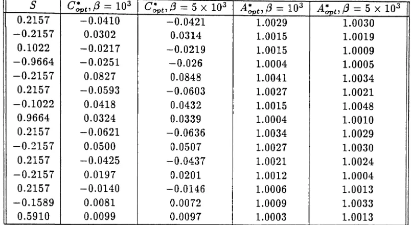
S _C~t,{3 == 103 C~t,(3 == 5X 103 A*_'Of}t,f3 _{- 10}3 A~t,_{{3 - 5 X 10}3

0.2157 -0.0410 -0.0421 1.0029 1.0030 -0.2157 0.0302 0.0314 1.0015 1.0019 0.1022 -0.0217 -0.0219 1.0015 1.0009 -0.9664 -0.0251 -0.026 1.0004 1.0005 -0.2157 0.0827 0.0848 1.0041 1.0034 0.2157 -0.0593 -0.0603 1.0027 1.0021 -0.1022 0.0418 0.0432 1.0015 1.0048 0.9664 0.0324 0.0339 1.0004 1.0010 0.2157 -0.0621 -0.0636 1.0034 1.0029 -0.2157 0.0500 0.0507 1.0027 1.0030 0.2157 -0.0425 -0.0437 1.0021 1.0024 -0.2157 0.0197 0.0201 1.0012 1.0004 0.2157 -0.0140 -0.0146 1.0006 1.0013 -0.1589 0.0081 0.0072 1.0009 1.0033 0.5910 0.0099 0.0097 1.0003 1.0013

20

Table 2: Optimal IS parameter vector 0~tfor the given mean vector S and a step size off3

=

103

and f3

==

5 X 103•

r

A/a-

P

~\{P} SPI I

V{P}

Sp

25.68 dB 1.532x10-6 _{4.332 X10-}13 _2.87X102 _6.542X10-1 7 _2.34X106

26.58 dB 1.116x10-7 _{8.05 X10-}1 5 _{8.96x1()2 2.845x10-}1 9 _{3.91 X10}7 27.21 dB 1.21x10-8 _{1.48 X10-}16 _4.5X103 _2.32X10-21 _5.2x108

27.70 dB 1.796x10-9 8.323 X10-18 5.57x1Q3 1.097x10-2 2 1.63 X109

Table 3: Simulation data and speed-up factors for the binary communication systemwith an RLS adaptive equalizer.

other hand, the same accuracy can be attained using only 16 decisions if the IS estimator of (7) is used and X is biased using e~t in Table 2 for

f3

==

5 X 103•

5

Conclusion

Stochastic Gradient Optimization ... , Al-Qaq, Devetsikiotis, and Townsend ₂₁

9 8

7

log ( 1/P)

6

0 ' - - - "

5

xlc1

Figure 4: A plot of the gain Sp]SPI versus log(l/

p).

noncoherent envelope detection, and a baseband communication system with a static linear

channel and an RLS equalizer. Speed-up factors of 2 to 10 orders of magnitude over

conven-tional Me were achieved for second and fourth order diversity systems, and of 6 to 9orders

of magnitude for the RLS adaptive equalization system for error probabilities in the range of 10-6 _{to 10-}9_.

References

[1] K. S. Shanmugan andP.Balaban. AModified Monte-Carlo Simulation Technique for the Evaluation of Error Rate in Digital Communication Systems. IEEE Trans. Commun., COM-28(11):1916-1924, Nov. 1980.

[2] D. Lu and K. Yao. Improved Importance Sampling Techniquefor Efficient Simulation ofDigital Communication Systems. IEEE J. Select. Areas Commun., 6(1), Jan. 1988.

Stochastic Gradient Optimization ... , Al-Qaq, Devetsikiotis, and Townsend ₂₂

[4] J-C. Chen, D. Lu, J. S. Sadowsky, and K. Yao. On Importance Sampling in Digi-tal Communications - Part I: Fundamentals. IEEE J. Select. Areas in Commun.,

11(3):289-299, Apr. 1993.

[5]

JC. Chen and J. S. Sadowsky. On Importance Sampling in Digital Communications -Part II: Trellis-Coded Modulation. IEEE J. Select. Areas in Commun., 11(3):300-308,

Apr. 1993.

[6] W. A. AI-Qaq, M. Devetsikiotis, and J. K. Townsend. Importance Sampling Method-ologies for Simulation of Communication Systems with Time- Varying Channels and Adaptive Equalizers. IEEE J. Select. Areas in Commun., 11(3):317-327, Apr. 1993.

[7] M. Devetsikiotis and J. K. Townsend. An Algorithmic Approach to the Optimization of Importance Sampling Parameters in Digital Communication System Simulation. IEEE

Trans. Commun., 41(10), Oct. 1993.

[8] M. Devetsikiotis and J. K. Townsend. Statistical Optimization of Dynamic Importance Sampling Parameters for Efficient Simulation of Communication Networks. IEEE/ACM

Trans. Networking, 1(3), June 1993.

[9] M. Devetsikiotis, W. AI-Qaq, J. A. Freebersyser, and J. K. Townsend. Stochastic Gra-dient Techniques for the Efficient Simulation of High-Speed Networks Using Importance Sampling. In Proc. IEEE Global Telecom. Coni., GLOBECOM '93, Houston, Dec. 1993.

[10] John

G.

Proakis. Digital Communications. New York: McGraw-Hill, 1989.

[11]

B. R. Davis. An Improved Importance Sampling Method for Digital Communication System Simulations. IEEE Trans. Commun., COM-34(7):715-719, Jul. 1986.

[12]

C. Nelson Dorny. A Vector Space Approach to Models and Optimization. New York:

Stochastic Gradient Optimization..., Al-Qaq, Devetsikiotis, and Townsend ₂₃

[13] P. W. Glynn. Stochastic Approximation for Monte Carlo Optimization. In Proc. ofthe Winter Simulation Conference, Wilson, J., Henriksen, J. and Roberts, S. (eds), IEEE Press, 1986.

[14] M. Metivier and P. Priouret. Applications of a Kushner and Clark Lemma to

Gen-eral Classes of Stochastic Algorithms. IEEE Trans. Inform. Theory,IT-30(2):140-151,

March 1984.

[15] S. S. Haykin. Adaptive Filter Theory. Englewood Cliffs, New Jersey: Prentice-Hall,

1986.

[16] P. W. Glynn. Likelihood Ratio Gradient Estimation: An Overview. In Proc. of the

Winter Simulation Conference, Thesen, A., Grant, H., Kelton, W. D., (eds), IEEE Press, 1987.

[17] P. W. Glynn. Likelihood Ratio Gradient Estimation for Stochastic Systems. Comm. ACM, 33(10):75-84, Oct. 1990.

[18] M. C. Jeruchim. Techniques for Estimating the Bit Error Rate in the Simulation of Digital Communication Systems. IEEE J. Select. Areas Commun., SAC-2(1):153-170,

Jan. 1984.

[19] John G. Proakis and Dimitris G. Manolakis. Digital Signal Processing. New York: Macmillan, 1988.

Appendix

In this Appendix, we justify the interchange of the gradient and expectation operators used

· (18) L t 0· (ll. ll* ll*]t Gl·ven the following assumptions:

ill . e ..

=

(]1'U2 ' ••·'U n •

1. 0 ~ I(X)

<

00,

2. I(X) is independent of the parameter vector 0*,

Stochastic Gradient Optimization ... , Al-Qaq, Devetsiliotis, and Townsend

4. wx(X,8,0*) is continuously differentiable with respect to 0*,

we need to show that

v e.Ee{l(X)wx(X,

0,

e*)} == Ee{l(X)V'

e.wx(X,

8,e*)}

Proof: It is only sufficient to show that for i == 1, ... ,n

aEe{I(X)wx(X,8, 8*)}

=

E. {Z(X) 8wx(X,

0, 0*)}

ao~\ e ao~

,

Applying the definition of the derivative, we get

24

(32)

(33)

aEe{I(X)wx(X, 8, 8*)}

=

lim Ee{I(X)wx(X,8, 8*)llJi =tii } - E{I(X)wx(X,8, 8*)}

8fJi 9~ -.8~_{, ,} {}~

,

- o~

,

Using assumption 3 , we can write

aEe{I(X)wX:X, 8, 8*)}

=

_lim E

e

{1(X)[WX(X,

8, 8*}llJi =tii - wx(X, 8, 8*)]}

ao;

_.

8~ -.8~, , IJ~

,

- IJ~

,

Applying the mean value theorem of calculus, we get

aEe{I(X)wx(X,8,8*)}

=

lim E_e

{1(X)8w

x

_{(X,e,e*)I . ,.}}

80* .. 80* 8. =8. ,

i 87-.87 i ' ,

Define

II

w

'11 -

- sup

{8w

x(X,

8f)*

0,

e*)

I

8!=8~

,}

X,0,0· i "

and

Illl/

== sup{l(X)}

X

By assumption 1, IIll/

<

00, and by assumption 4,

Ilw'll

<

00. Therefore, we may write

leX)

awx(~~~8,

8*)1lJi=tii

~

Illllllw'll

<

00,

I

Thus, we can apply the Lebesgue Dominated Convergence Theorem (DCT)

.

{

8wx(X,

8, 8*) } _ { .

8wx(X,

8,(3*) }

i~i

Ee leX) a(J: 1lJi=tii -

s,

leX)

tiP3

i a(J: 1lJi=tii

_ E

_a

{1(X)

awx(~~i8,

0*)}

(34)