Stepwise Hypothesis Testing with Applications in Pharmaceutical Responses

(1)

ABSTRACT

GAUVIN, JENNIFER LYNN SHANNON. Stepwise Hypothesis Testing with

Appli-cations in Pharmaceutical Responses. (Advisor: Dr. Roger L. Berger)

In some studies researchers seek to identify conditions under which a mean response

exceeds a specified threshold. This work examines the case in which such conditions are

defined in terms of two quantitative independent variables. For example, a

pharmaceu-tical researcher might want to identify what values of dose and post-dose time yield an

average blood concentration above a certain threshold.

New methods of specifying a rectangular set of (time,dose) values for which the

researcher can assert that the mean response exceeds the threshold are described. By

using intersection-union tests applied in a stepwise fashion, the methods maintain a

specified high probability that the rectangular set contains no (time,dose) values for

which the mean response is lower than the threshold.

The observations at each (time,dose) value must be independent, but neither method

requires independent observations at different (time,dose) values. For example,

concen-trations measured on a subject at different time points may be correlated.

Exact calculations and simulation studies are used to assess the error rates and

(2)

STEPWISE HYPOTHESIS TESTING WITH APPLICATIONS IN PHARMACEUTICAL RESPONSES

by

Jennifer Lynn Shannon Gauvin

A dissertation submitted to the Graduate Faculty of

North Carolina State University

in partial fulfillment of the requirements for the

Degree of Doctor of Philosophy

DEPARTMENT OF STATISTICS

Raleigh, NC

2003

APPROVED BY:

Roger L. Berger Dennis D. Boos

Chair of Advisory Committee

(3)

Dedication

(4)

Biography

Jennifer Lynn Shannon Gauvin was born in Warren, Ohio on September 20, 1973. She

received a Bachelor of Science degree in Interdisciplinary Mathematics: Statistics from

the University of New Hampshihre in 1995. After a year, Jennifer enrolled in graduate

school at North Carolina State University in the Department of Statistics. In 1998, she

received a Master of Statistics degree from North Carolina State University. Jennifer

continued her studies in statistics, completing her doctoral degree in 2003 from North

(5)

ACKNOWLEDGEMENTS

I am grateful and honored to have had the privilege of working with my advisor, Dr.

Roger L. Berger. Without his expertise, guidance and patience this dissertation would

not be complete.

Thank you to my committee members Drs. Dennis Boos, Bill Swallow and Butch

Tsiatis for your suggestions and teaching during my education. Dr. Sastry Pantula,

thank you for teaching me essential study tips and test taking strategies. I appreciate

how freely you gave your time despite your full schedule.

Thank you to Wendy Czika, Buffy Hudson-Curtis and Steve Novick for their valuable

support during my graduate studies.

Over my many years as a student I have learned from my fellow students and

col-leagues. Hearing their insightful comments and observing their approaches to statistical

challenges has made me a better statistician.

I am very fortunate to have amazing people in my life who encouraged and supported

me throughout this entire experience. I cannot thank them enough.

To my parents, Raymond and Marsha Shannon, thank you for teaching me the value

of diligence. To my sisters, Hilary and Heather, and my brother and sister-in-law, Michael

and Allyson, thank you for listening to all my trials and adventures. To my husband,

(6)

List of Tables

1.1 Points tested in each of the four regions at steps 1 and 2. . . 9

2.1 The points tested at each step in each region of a 7×7 grid. . . 22 2.2 Step 1: Snapshot of data points surrounding the initial point in Pattern D. 47

2.3 Step 2: Adaptive algorithm snapshot of data points for Pattern D. . . . 48

2.4 Step 3: Adaptive algorithm snapshot of data points for Pattern D. . . . 49

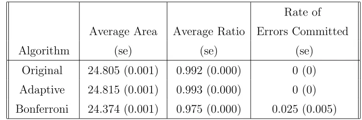
3.1 1000 simulations of the rectangle shape. Standard errors are listed in

parentheses. . . 58

3.2 1000 simulations of the ridge shape. Standard errors are listed in

paren-theses. . . 61

3.3 1000 simulations of the dome shape. Standard errors are listed in

paren-theses. . . 65

3.4 The largest rectangular set under the Bonferroni method in 100

simula-tions of each shape using the parameters in Secsimula-tions 3.2.1, 3.2.2 and 3.2.3.

(9)

3.5 1000 simulations of the rectangle shape with the initial point (5,5).

Stan-dard errors are listed in parentheses. Results from the initial point (4,4)

are given in Table 3.1. . . 72

3.6 1000 simulations of the ridge shape with the initial point (4,3). Standard

errors are listed in parentheses. Results from the initial point (4,4) are

given in Table 3.2. . . 74

3.7 1000 simulations are run to study the effect of µ and grid size on the

Bonferroni method. Standard errors are listed in parentheses. . . 77

3.8 1000 simulations show an error rate near 5% for Original and Adaptive

methods. Standard errors are listed in parentheses. . . 82

3.9 Correlation between pairs of observations in an AR(1) model. . . 85

3.10 1000 simulations of the rectangle shape with AR(1) correlated data.

Stan-dard errors are listed in parentheses. . . 86

3.11 1000 simulations of the ridge shape with AR(1) correlated data. Standard

errors are listed in parentheses. . . 87

3.12 1000 simulations of the dome shape with AR(1) correlated data. Standard

(10)

List of Figures

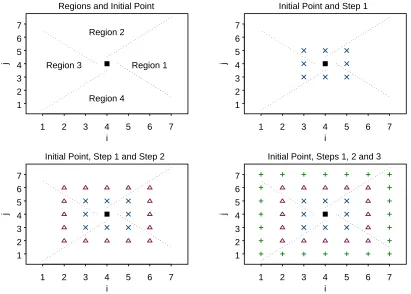
1.1 Regions and steps in the Original algorithm . . . 7

2.1 The asymmetric shape is trimmed into a rectangular set. . . 23

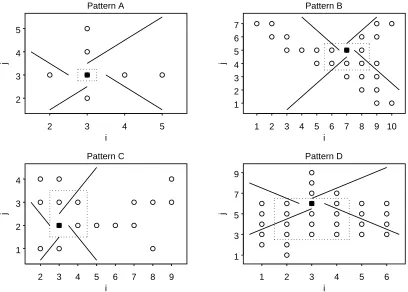
2.2 Patterns which are difficult to detect. The Original algorithm finds the

rectangular set in the dotted lines. . . 39

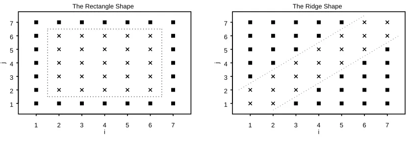
3.1 The rectangle and ridge shapes. µ >0 for points marked by ×. µ= 0 for points marked by squares. . . 60

3.2 The dome shape. The vertical axis represents values of µij. . . 64

3.3 The rectangle shape with initial point (5,5). µ = 1 for points marked by

×. µ= 0 for points marked by squares. The initial point is marked with a diamond. Regions are separated by solid lines. Rectangular sets are

(11)

3.4 The ridge shape with initial point (4,3). µ > 0 for points marked by ×.

µ = 0 for points marked by squares. The initial point is marked with a

diamond. Regions are separated by dotted lines. The rectangular set is

outlined with dotted lines. . . 75

3.5 This shape is constructed to demonstrate that the Adaptive method

(12)

Chapter 1 Overview

1.1 Introduction

In many studies, researchers may seek to identify a set of conditions for which the

popula-tion quantity exceeds a desired threshold,δ. The population quantity,µfor example, may

depend on quantitative factors or conditions, such as time or drug dosage. Correlation

may exist between the observations at the same dose and different time points.

While it is interesting to explore the values of µ, this research places additional focus

on compiling a useful set of conditions for which the confidence statement,µexceeds the

threshold, can be asserted. These conditions are the set of values for the independent

variables, time and drug dosage. Ultimately, a collection of (time,dose) pairs will describe

the region where the confidence statement is valid. The region will consist of pairs,

(13)

pairs of values.

The region must be easy to understand and interpretable. Suppose the region is

{(1,1),(5,5),(3,2)}. The corresponding confidence statement, using this region, is µ

exceeds the threshold at 1 hour for 1 mg, at 5 hours for 5 mg and at 3 hours for 2 mg.

There is no pattern in the pairs. Suppose the region is{(1,1),(1,2),(1,3),(1,4),(1,5)}. The confidence statement isµ exceeds the threshold at 1 hour for doses 1, 2, 3, 4, and 5

mg. The pattern in these pairs is clear.

If drawn on a grid, the second collection of points produces a line or rectangle of

adjacent pairs. The pairs in the first example do not take any simple shape. Keeping

in mind the grid framework, the rectangle has appeal because of the simple statements

which can be made. Clear, concise statements describe the rectangle. For example, {

a≤time≤b and c≤dose≤d } describes a rectangle.

Confidence statements are constructed for parameters. This research explores the

val-ues of the independent variables for which confidence statements about µ are asserted.

Values of independent variables depend on the variable and its application

(pharma-ceutical, industrial, otherwise). As described, a collection of desirable pairs is found.

Further, the region of points (time,dose) will adhere to a rectangular pattern. With

these requirements, the final result is more meaningful to the application.

The region will contain the set of (time,dose) pairs for the confidence statement that

the population quantity µexceeds the threshold δ. The proposed methodology does not

(14)

to those at 2 hours for dose =c.

Simultaneous inferences are required to test and assert a condition such as µ > δ for

dose d1 at time points t1, t2, and t3. This statement can be rewritten as an intersection of three distinct statements {µ > δ at (time = t1,dose = d1) and µ > δ at (time =

t2,dose = d1) and µ > δ at (time = t3,dose = d1)}. Often, simultaneous inferences re-quire multiplicity adjustments. Unfortunately, such adjustments can lead to conservative

estimates of error.

Using the intersection-union method and stepwise hypothesis testing, the overall

sig-nificance level of the test is controlled without multiplicity adjustments. In stepwise

hypothesis testing, test hypotheses are ordered a priori such that testing continues in a

sequence if and only if significance is found at the previous step. As an example, consider

the hypotheses

H01:µ≤δ for at least one (t, d) such that d∈ {d1} and t∈ {t1, t2, t3}

Ha1 :µ > δ for all (t, d) such that d∈ {d1} and t∈ {t1, t2, t3} and

H02 :µ≤δ for at least one (t, d) such that d∈ {d1, d2} and t∈ {t1, t2, t3}

Ha2 :µ > δ for all (t, d) such that d∈ {d1, d2} and t ∈ {t1, t2, t3}.

The null hypothesis H01 tests the parameter µ. Its alternative, Ha1, will be asserted at

(15)

If the test fails to reject H01, clearly H02 will also fail to be rejected. If the test for

H01 is significant, there is a chance that the test for H02 may also be significant. Test

H02 if and only if H01 is rejected. IfH01 is not rejected, there is no reason to test H02. With each step of testing, more points are included in the region. In the previous

example, µ is tested at three (time,dose) points in the first step with null hypothesis

H01. In the second step, H02, µ is tested at the same three points and three additional points.

The methods proposed in this work do not retest points at sequential hypotheses as

is done in the previous example. Points farther from the initial point are tested in steps,

increasing the number of points tested at each step, expanding the testing away from the

initial point. Stepwise testing protects the confidence region from being unnecessarily

conservative.

1.2 Historical Background

Prior to this research, Berger and Boos addressed the same question. However, their

research only allowed for one independent variable (Berger and Boos 1999). Using time

as an example, they concludedµ > δfor all timetsuch thatt∈[t1, t2]. In brief summary, they chose a point, tap, such that 0 ≤ tap ≤ tn, where tn is the longest time available.

Using stepwise methods, they assertµ > δfor allt ∈[t1, tap) andµ > δfor allt∈(tap, t2].

Using Bonferroni’s inequality, the information in these separate pieces can be combined

(16)

Berger and Boos laid a careful foundation for further studies. This research seeks to

construct a 100(1−α)% confidence statement forµ,µ > δ for all (i, j)∈ {a≤i≤b, c≤

j ≤d}. Here, two independent variables, Aand B, are under simultaneous consideration with levels of A represented by i = 1, . . . , I and levels of B represented by j = 1, . . . , J.

Using the previous example, A would correspond to time and B would correspond to

dose. If one of the two independent variables is set to a fixed value, the situation is a

case of Berger and Boos’ work. For example, µ > δ for all (i, j)∈ {a≤i≤b, j =c}. In order to discuss confidence statements, the type I error must be clearly defined. A

type I error occurs if the set {a ≤i≤b, c≤j ≤d} contains any (i, j) at which µij ≤δ.

The probability of committing a type I error is at most α; the probability that the set

{a≤i≤b, c≤j ≤d} contains any (i, j) with µij ≤δ is at most α.

A first step in this research is to determine how, if at all, to apply Bonferroni’s

inequality. Having information about the values of the independent variables is essential.

For example, if each variable takes only two values, the largest possible region of paired

independent variable values contains four points, for example,{(1,1),(1,2),(2,1),(2,2)}. Testing µat each (i, j) point with level α

4 seems reasonable and simple. However, if each independent variable can take one of ten values, it seems naive to test µ at each (i, j)

point with level α

100. Using such a small significance level will lead to very conservative results and, quite possibly, a strangely shaped region which is meaningless in applications.

Consider the a priori element of Berger and Boos’ method. They begin their study

(17)

information about the application or past data. The choice of an initial point is somewhat

arbitrary, but should be made carefully and thoughtfully with intent that the initial point,

(iap, jap), will be in the set.

With one independent variable, there are two directions around the initial point,

right or left. Berger and Boos apply Bonferroni’s inequality and construct two intervals,

each having error probability α

2. With two independent variables, there are four direc-tions around the initial point, right, up, left or down. Applying Bonferroni’s inequality

to a method which constructs four regions around the initial point, each having error

probability α

4, will produce a rectangular set having error probabilityα.

Consider a sequential manner for testing µ at points within each of the four regions.

For Region 1, test points to the right of the initial point. For Region 2, test points above

the initial point. For Region 3, test points to the left of the initial point. For Region

4, test points below the initial point. Overlap can be avoided by assigning upper right

points to Region 1, upper left points to Region 2, lower left points to Region 3 and lower

right points to Region 4. The null and alternative hypotheses are, in general,

H0 :µ≤δ for at least one (i, j) in the described set

Ha:µ > δ for all (i, j) in the described set.

The described set of (i, j) in the hypotheses depends on the region and the sequential

step, which are illustrated in Figure 1.1. These tests, which are intersection-union tests,

have properties beneficial to this work. Details are provided in later sections. The null

(18)

Regions and Initial Point

i

j

1 2 3 4 5 6 7

1 2 3 4 5 6 7 Region 1 Region 2 Region 3 Region 4

Initial Point and Step 1

i

j

1 2 3 4 5 6 7

Initial Point, Step 1 and Step 2

i

j

1 2 3 4 5 6 7

Initial Point, Steps 1, 2 and 3

i

j

1 2 3 4 5 6 7

(19)

intersection of statements. These hypotheses could be rewritten as follows to explicitly

demonstrate this characteristic. Suppose the described set is {i = 1 and j = 1 or 2}. Then, the hypotheses are

H0 :{µ≤δ for (1,1)} or{µ≤δ for (1,2)}

and

Ha:{µ > δ for (1,1)}and {µ > δ for (1,2)}.

Stepwise testing is utilized to limit multiplicity adjustments. If the test is significant

at the first step, testing can continue to the second step. If testing is not significant

at step 1, further testing will not occur. Since an initial point is selected, each point

immediately adjacent to the initial point will be tested in the first steps. Testing will

occur in the four regions which are described in Figure 1.1. In the first step, each point

immediately adjacent to the initial point will be tested in one of four regions. Suppose

the initial point is (iap, jap), where 1 ≤ iap ≤ I and 1 ≤ jap ≤ J. For the independent

variable A, iap+ 1 represents one level greater than iap and iap−1 represents one level

smaller than iap. For example, if i = 1,2,3,4,5 and iap = 3 then iap + 1 = 4 and

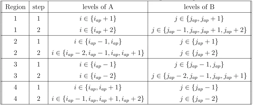
iap−1 = 2. Steps 1 and 2 are described in Table 1.1 for each of the four regions.

The proposed method maintains an overall significance level ofα, but hypothesis

test-ing at each grid point, except the initial point, is performed at level α

4. Stepwise testing requires no adjustment. The test for Region 1, step 1 has the same error probability

as the test for Region 1, step 2 and so on. This method of testing is not

(20)

Table 1.1: Points tested in each of the four regions at steps 1 and 2.

Region step levels of A levels of B

1 1 i∈ {iap+ 1} j ∈ {jap, jap+ 1}

1 2 i∈ {iap+ 2} j ∈ {jap−1, jap, jap+ 1, jap+ 2}

2 1 i∈ {iap−1, iap} j ∈ {jap+ 1}

2 2 i∈ {iap−2, iap−1, iap, iap+ 1} j ∈ {jap+ 2}

3 1 i∈ {iap−1} j ∈ {jap−1, jap}

3 2 i∈ {iap−2} j ∈ {jap−2, jap−1, jap, jap+ 1}

4 1 i∈ {iap, iap+ 1} j ∈ {jap−1}

4 2 i∈ {iap−1, iap, iap+ 1, iap+ 2} j ∈ {jap−2}

increases as well. While this does not make it more difficult to detect significance at

individual points, it does become more difficult to find large sets of points where the

test is significant at each (i, j) point. As the described sets become larger, the number

of points simultaneously tested in a null hypothesis increases. Recall, the test at each

of the points must be significant in order to reject the null hypothesis for the step. If

the test at any of the points fails to reject the null hypothesis the stepping stops; the

rectangular set will not expand.

The ideas in this section are a small subset of what has been explored. Issues of

concern that ultimately affected the final solution are the ability to find the largest

possi-ble region under feasipossi-ble data trends with respect to independent variapossi-bles, conservative

significance levels for testing, patterns for testing such as the rectangle and theoretical

(21)

Chapter 2 A New Problem

2.1 Introduction

The focus of this work is to construct a 100(1−α)% confidence statement for the mean parameter at all points in the rectangular set of pairs of independent variable values. In

general, for two independent variables, A and B, let µij represent the population mean

at the ith _{level of} _A _{and the} _jth _{level of} _B_. _A _has _I _{levels, with} _i _{= 1}_{, . . . , I}_{, and} _B

has J levels j = 1, . . . , J. The levels of each factor must be ordered. In the example in

Section 1.1, A denoted time and B denoted dose. The levels of A must be in increasing

or decreasing order such as{5,10,20,50}or {50,20,10,5} minutes. Similarly, the levels of B must be in increasing or decreasing order such as {3,10,13,20} or {20,13,10,3} mg. The levels need not be equally spaced.

(22)

the ith _{level of A and the}_jth _{level of B. Here,}_ǫ

ijk represents the error of thekth response

with k = 1, . . . , nij. The errors are identically distributed normal random variables at

each (i, j) level; ǫijk ∼ N(0, σij2). Errors are independent at each (i, j) level, but need

not be independent between (i, j) levels. This model differs from a two-way anova model

because the independent variables are order restricted and observations may have unequal

variances. Ordering necessary for stepwise testing will be discussed later.

As mentioned previously, the set of (i, j) pairs for which the mean exceeds the

thresh-old δ must be efficacious and practical. A rectangular set meets these requirements and

will be utilized in this research. The set of (i, j) pairs can be fully described and explained

by a rectangular set such as all (i, j) where {a≤i≤b and c≤j ≤d}.

For this research, constructing the rectangular set will begin with an initial (i, j) pair

chosena priori, before the data are observed. The initial point, (iap, jap), should be chosen

based on the application, previous data, previous studies or desirable characteristics.

Naturally, research will be most productive if the initial point is expected to be in the

final rectangular set.

A t-test of H0 :µiapjap ≤δ, performed at the initial point, should reject H0 if

y_i_ap_j_ap −δ

r

s2

iapjap

niapjap

> t(1−α),(niapjap−1).

A t-test of H0 :µij ≤δ, performed at any other grid point, should reject H0 if

yij−δ

r

s2

ij

nij

(23)

Notice, the significance level, α, at the initial point. The algorithm has greater chance of

rejecting the null hypothesis and beginning the stepwise process at the initial point than

at each subsequent step where the level is more conservative, α

4.

In keeping with traditional definitions, the sample variance of observations at (i, j) is

defined as

s2_ij = 1

nij −1 nij

X

k=1

(yijk−yij.)2

and the sample mean is

y_ij = 1

nij nij

X

k=1

yijk .

The variance estimate has not been pooled because there is no assumption of

ho-moscedasticity. That is, the estimated variance at each (i, j) depends only on the nij

observations at (i, j). A pooled estimate of variance would be calculated for data which

assumes homoscedasticity. The pooled estimate of variance is presented in the following

formula.

s2 = _P_I 1

i=1

PJ

j=1(nij −1) I X i=1 J X j=1

(nij −1)(s2ij)

= 1

(PI

i=1

PJ

j=1nij)−IJ I X i=1 J X j=1 nij X k=1

(yijk−yij.)

2_.

Recall the grid of points, Figure 1.1, as described in Section 1.2. At any one (i, j) grid

point, there are nij observations. Building on the example from Section 1.1, suppose A

takes values {5,10,15,30,45,60,75}minutes, then i= 1 corresponds to A at 5 minutes. Similarly, i = 5 corresponds to A at 45 minutes. Further, suppose B takes values

(24)

corresponds to B at 30 mg. In this example, the (i, j) pair at (1,5) corresponds to data

observed at 5 minutes for 30 mg.

This section outlines the research problem and proposes ideas about finding a

solu-tion or result. The remainder of Chapter 2 explains, in detail, methods which answer

the research problem. In Section 2.2, the method for constructing the rectangular set

is defined. Error probability is discussed in Section 2.3. Potential problems with the

Original method from Section 2.2 are discussed in Section 2.4. The Adaptive method is

described in Section 2.5; in addition, the distinction between the Adaptive and Original

algorithms is made clear by contrasting the benefits of each process.

2.2 The Original Method of Constructing a

Rectan-gular Set

The experimental goal is to answer the question at which doses for which time points

does the population mean exceed a desired threshold. This section explains how a set

of pairs of doses and times will be constructed in answer to the experimental question.

Details in this section will be given in terms of (i, j) pairs that represent the levels of

time and dose levels. The method of constructing the rectangular set of (i, j) points,

{a≤i≤b and c≤j ≤d}, will be described in this section. Proof of how the algorithm maintains a specified error probability of α and an explanation of how the algorithm

(25)

A 7×7 grid will be used to illustrate how the set is constructed. After describing the method for the specific example of a 7×7 grid, detailed steps will be outlined for the general case, an I×J grid. The regions and steps are illustrated on a 7×7 grid in Figure 1.1.

An initial point must be chosen to begin constructing a set of (i, j) pairs where the

100(1−α)% confidence statement is valid for the population mean. Recall that the choice

is made a priori. If no information suggests otherwise, choose (4,4), the center point of

a 7×7 grid for the initial point. The choice of initial point can greatly affect the success or failure of constructing the rectangular set. The algorithm must recover from a poor

initial choice and benefit from a wise initial choice.

To begin, a t-test of H0 : µ4,4 ≤ δ againstHa : µ4,4 > δ is performed using all n4,4 observations at the initial point (4,4). The t-test should reject H0 if

y₄_,₄−δ

q

s2 4,4

n4,4

> t(1−α),(n4,4−1).

If the test fails to reject the null hypothesis, no further tests will be performed; no set can

be found based on the initial start value (4,4). If the test rejects the null hypothesis, the

procedure of hypothesis testing will continue. Assuming the test rejects, the algorithm

can assert that the mean exceeds the desired threshold at (4,4) with error probabilityα.

Next, consider expanding the set, now {(4,4)}, to include more points. The choice for direction of expansion is arbitrary. Recall the method of expansion introduced in

Section 1.2. Consider grouping the points around the initial point into four regions. The

(26)

using points where j > jap. The third group is constructed using points where i < iap.

The fourth group is constructed using points where j < jap.

Hypothesis testing will be done in steps within each region. The hypothesis tested at

step 1 in the first group is

H₀₁1 :µij ≤δ for at least one (i, j)∈ {(5,4),(5,5)}

against

H_a1₁ :µij > δ for all (i, j)∈ {(5,4),(5,5)}.

These points, {(5,4),(5,5)}, are represented in Figure 1.1 of Section 1.2 in Region 1. The null hypothesis can be rejected if and only if the t-test is significant at both

(5,4) and (5,5). For (5,4), if

y₅_,₄−δ

q_s2 5,4

n5,4

> t(1−α4),(n5,4−1) (2.1)

and for (5,5), if

y₅,5−δ

q_s2 5,5

n5,5

> t(1−α4),(n5,5−1) (2.2)

then reject H₀₁1 , the null hypothesis for the first step in the first region. If either test is

not significant,H1

01fails to be rejected and the expansion halts in the direction of the first group. This also signifies a boundary or border for the final rectangular set; by design,

no point in the final set will have i >4.

The null hypothesis, H1

01, can be written as a union of two statements which can be tested by two hypotheses. H₀₁₁1 : µij ≤ δ for (i, j) ∈ {(5,4)} or H0121 : µij ≤

(27)

represent the null hypothesis for the first point at the first step in the first region,

{(5,4)}. Similarly, let H1

012 represent the null hypothesis for the second point at the first step in the first region, {(5,5)}. Using the same notation, the alternative can be written as H_a1₁ : {µij ≤δ for at least one (i, j) ∈ {(5,4),(5,5)}}c which is equivalent to

H1

a11 : µij > δ for (i, j) ∈ {(5,4)} and Ha112 : µij > δ for (i, j) ∈ {(5,5)}. In order to

assert the alternative hypothesis and reject H1

01, both H0111 and H0121 must be rejected. The rejection region forH₀₁1 isR₁1 =R1₁₁T

R₁₂1 , where R1₁₁ is the rejection region defined by Equation 2.1 and R1

12 is the rejection region defined by Equation 2.2.

R1₁₁ and R₁₂1 are each level-α

4 rejection regions of H 1

011 and H0121 , respectively. By the intersection-union test method, it follows that R1₁ = R1₁₁T

R₁₂1 is the level-α

4 rejection region of H1

01 (Casella and Berger 2002). The intersection-union test method requires no multiple test adjustment.

Assuming H₀₁1 was rejected, the algorithm can assert that the mean exceeds the

desired threshold at points {(4,4),(5,4),(5,5)}. The rejection region at the initial point is a level-α region and the rejection region for step 1 in Region 1, {(5,4),(5,5)}, is a level-α

4 rejection region. A full explanation of error probability is given in Section 2.3. Stepwise expansion in the direction of the first group, continues in step 2 by examining

data at points {(6,3),(6,4),(6,5),(6,6)}. In Figure 1.1 from Section 1.2, these points are represented by triangles in Region 1. The hypothesis tested at step 2 for the first

region is

(28)

against

H_a1₂ :µij > δ for all (i, j)∈ {(6,3),(6,4),(6,5),(6,6)}.

The null hypothesis can be rejected if and only if the t-test is significant at each

(i, j)∈ {(6,3),(6,4),(6,5),(6,6)}. For each (i, j) in this group, if

y_ij −δ

r

s2

ij

nij

> t(1−α4),(nij−1)

then rejectH1

02, the null hypothesis for the second step in the first group. If the t-test at any of the four points is not significant, H₀₂1 fails to be rejected and the expansion halts in the first group.

The null hypothesis, H1

02, can be written as a union of four statements. There is one hypothesis for each test point. H₀₂₁1 : µij ≤ δ for (i, j) ∈ {(6,3)} or H0221 : µij ≤

δ for (i, j) ∈ {(6,4)} or H₀₂₃1 : µij ≤ δ for (i, j) ∈ {(6,5)} or H0241 : µij ≤ δ for (i, j) ∈

{(6,6)}. H1

021 represents the null hypothesis for the first point at the second step in the first region. H₀₂₂1 represents the null hypothesis for the second point at the second step in the first region. H₀₂₃1 represents the null hypothesis for the third point at the second

step in the first region. Similarly,H1

024 represents the null hypothesis for the fourth point at the second step in the first region.

Using the same notation, the alternative can be written as H_a1₂ :{µij ≤δ for at least

one (i, j) ∈ {(6,3),(6,4),(6,5),(6,6)}}c _{which is equivalent to} _H1

a21 : µij > δ for (i, j)∈

{(6,3)} and H_a1₂₂ :µij > δ for (i, j)∈ {(6,4)} and Ha123 :µij > δ for (i, j)∈ {(6,5)} and

(29)

and only if the hypotheses H₀₂₁1 and H₀₂₂1 and H₀₂₃1 and H₀₂₄1 are all rejected.

The rejection region for H1

02 isR21 =R121

T R1 22 T R1 23 T R1

24, where R121, R122,R231 and

R1₂₄are the level-α

4 rejection regions ofH 1

021, H0221 , H0231 , and H0241 . The intersection-union test method requires no multiple test adjustment so R1₂ is a level-α

4 rejection region of

H1

02. Error probabilities are discussed in Section 2.3. Assuming H1

02 was rejected, the algorithm can now assert that the mean exceeds the desired threshold at points

{(4,4),(5,4),(5,5),(6,3),(6,4),(6,5),(6,6)}.

At step 3 in Region 1, the null hypothesis is

H₀₃1 :µij ≤δ for at least one (i, j)∈ {(7,2),(7,3),(7,4),(7,5),(7,6),(7,7)}

against

H_a1₃ :µij > δ for all (i, j)∈ {(7,2),(7,3),(7,4),(7,5),(7,6),(7,7)}.

The null hypothesis can be rejected if and only if the t-test is significant at each (i, j)∈ {(7,2),(7,3),(7,4),(7,5),(7,6),(7,7)}. For each (i, j) in this group, if

yij −δ

r

s2

ij

nij

> t(1−α4),(nij−1)

then reject H₀₃1 , the null hypothesis for the third step in the first region. If the t-test at any of the six points is not significant, H₀₃1 fails to be rejected and the expansion halts

(30)

The null hypothesis, H₀₃1 , can be written as a union of six statements. There is one

hypothesis for each of the six test points at this step. These points,

{(7,2),(7,3),(7,4),(7,5),(7,6),(7,7)},

are represented in Figure 1.1 of Section 1.2 with + (plus) signs. The alternative is

literally,

H_a1₃ :{µij ≤δ for at least one (i, j)∈ {(7,2),(7,3),(7,4),(7,5),(7,6),(7,7)}}c,

which is equivalent to

H_a1₃ :µij > δ for every(i, j)∈ {(7,2),(7,3),(7,4),(7,5),(7,6),(7,7)}.

The alternative hypothesis, H1

a3, can be asserted if and only if the null hypotheses at each (i, j) is rejected.

The rejection region for H₀₃1 is R1₃, a level-α

4 rejection region. Assuming H 1 03 was rejected, the algorithm can assert that the mean exceeds the desired threshold at points

from each step in Region 1:

initial point { (4,4),

step 1 (5,4),(5,5),

step 2 (6,3),(6,4),(6,5),(6,6),

step 3 (7,2),(7,3),(7,4),(7,5),(7,6),(7,7) }.

To find the full set of points where the mean exceeds the desired threshold the

algo-rithm must step through the three other regions. In each region, the first step consists

(31)

In the second region, j > jap. This region is depicted in Figure 1.1 in Section 1.2.

The hypothesis test at step 1 in Region 2 is

against

H_a2₁ :µij > δ for all (i, j)∈ {(3,5),(4,5)}.

These points, {(3,5),(4,5)}, are represented in Figure 1.1. The algorithm advances to the next step if and only if the intersection-union test rejects H2

01. The data points to examine in step 2 are

{(2,6),(3,6),(4,6),(5,6)}.

Similarly, if the algorithm reaches the third step, H₀₃2 is a union of six statements. There is one hypothesis for each of the six test points described by{(i, j) : 1 ≤i≤6 andj = 7}. For Region 2, the group of (i, j) tested in step 1 can be described by j = 5 and 3≤

i ≤ 4. The set of (i, j) in step 2 can be described as (i, j) where j = 6 and 2 ≤ i ≤ 5. Similarly, the set of points for the third step can be described as (i, j) where j =

7 and 1≤ i≤6.

Recall, the third region is characterized byi < iap. In the third region, the hypothesis

test at step 1 is

against

(32)

For the third region, the set of (i, j) in step 1 is all (i, j) where i= 3 and 3≤j ≤4. The set of (i, j) in step 2 can be described as (i, j) where i= 2 and 2≤j ≤5. Similarly, the set of points for the third step can be described as (i, j) where i= 1 and 1≤j ≤6.

The fourth region is characterized by j < jap. In the fourth and final region, the

hypothesis tested at step 1 is

against

H_a4₁ :µij > δ for all (i, j)∈ {(4,3),(5,3)}.

The set of (i, j) in step 1 is all (i, j) where j = 3 and 4≤i≤5. The set of (i, j) in step 2 can be described as (i, j) where j = 2 and 3 ≤ i ≤ 6. Similarly, the set of points for the third step is all (i, j) where j = 1 and 2≤i≤7.

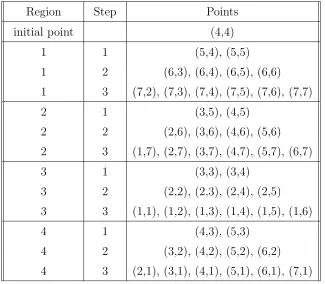
Using this 7×7 example, a summary of the algorithm for each step in each region is listed in Table 2.1. This example demonstrates how the procedure would test all the

data in a 7×7 grid, beginning with the initial point at the center, (4,4). In review, the overall grid is divided into four regions. Within each region, data is tested in a series

of steps. The hypothesis test at each step is an intersection-union test for two or more

points. Each sequential step tests data farther from the initial point than its previous

step; each step is one i orj unit farther from the initial point than the previous step.

For example, including all regions, step 2 forms a box around step 1. In Figure 1.1 of

(33)

Table 2.1: The points tested at each step in each region of a 7×7 grid.

Region Step Points

initial point (4,4)

1 1 (5,4), (5,5)

1 2 (6,3), (6,4), (6,5), (6,6)

1 3 (7,2), (7,3), (7,4), (7,5), (7,6), (7,7)

2 1 (3,5), (4,5)

2 2 (2,6), (3,6), (4,6), (5,6)

2 3 (1,7), (2,7), (3,7), (4,7), (5,7), (6,7)

3 1 (3,3), (3,4)

3 2 (2,2), (2,3), (2,4), (2,5)

3 3 (1,1), (1,2), (1,3), (1,4), (1,5), (1,6)

4 1 (4,3), (5,3)

4 2 (3,2), (4,2), (5,2), (6,2)

(34)

1 2 3 4 5 6 1 2 3 4 5 6 i j

Pairs found, separated by Region, Initial Point highlighted

1 2 3 4 5 6

1 2 3 4 5 6 i j

Rectangular Set after trimming, five points excluded

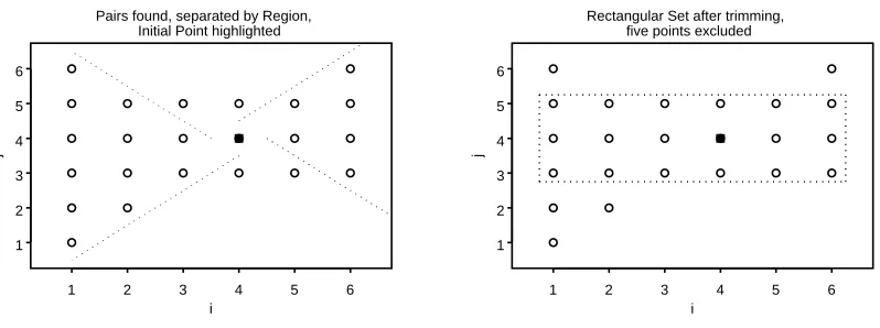
Figure 2.1: The asymmetric shape is trimmed into a rectangular set.

points are tested only once. For example, the upper right corner is assigned to Region 1,

but it is not assigned to Region 2. Similarly, the upper left corner is assigned to Region

2. The lower left corner is assigned to Region 3 and the lower right corner is assigned to

Region 4.

In reality, this procedure may not encounter complete success. The algorithm may

not proceed through all three steps in all four regions for every data example. Suppose

a test fails to reject the null hypothesis in a region at a step. In this case, the final set

may look more asymmetric than rectangular. Figure 2.1 depicts an example in which the

algorithm finds only the points that are marked.

In words, the points depicted in Figure 2.1 are the initial point and points from Region

1 at steps 1 and 2, Region 2 at step 1, Region 3 at steps 1, 2 and 3 and Region 4 at step

1. The largest possible rectangle within this shape can be described by the set of (i, j)

(35)

easily interpretable shape, a rectangular set.

Trimming the points is handled within each region by retaining maximum or minimum

values. For the first region, step testing occurs by increasing the value ofiand varying the

values of j with each step. Upon the last successful step in the first region, a maximum

value will be stored for i, imax. For the second region, step testing occurs by increasing the value of j and varying the values of i with each step. Upon the last successful step

in the second region, a maximum value will be stored for j, jmax. For the third region,

step testing occurs by decreasing the value of i and varying the values of j with each

step. Upon the last successful step in the third region, a minimum value will be stored

for i, imin. For the fourth region, step testing occurs by decreasing the value of j and

varying the values of iwith each step. Upon the last successful step in the fourth region,

a minimum value will be stored forj,jmin. Having stored minimum and maximum values for i and j, the procedure can report that the mean exceeds the desired threshold δ at

each of the points in the rectangular set of{(i, j) :imin ≤i≤imax and jmin ≤j ≤jmax}. Thus far, the method for answering the research question, at which doses for which

time points does the population mean exceed a desired threshold, has been described by

example. The detailed steps must be documented for a general I×J grid.

An initial point must be chosen a priori. Let (iap, jap) be the initial point. There

are no restrictions on the initial point, so, (iap, jap) may be equal to (I, J) or (1,1), for

(36)

niap,jap observations at the initial point (iap, jap). The t-test should reject H0 if

y_i_ap_,j_ap−δ

r

s2

iap,jap

niap,jap

> t(1−α),(niap ,jap−1).

If the test fails to reject the null hypothesis, no further tests will be performed; no

rectangular set can be constructed based on the initial start value (iap, jap). If the test

rejects the null hypothesis, the algorithm can assert that the population mean exceeds

the desired threshold at {(iap, jap)} with probability of an error no more than α. The

procedure of hypothesis testing will continue.

Begin expanding the set, now {(iap, jap)}, by testing points in Region 1 where i > iap.

If iap < I there are I −iap potential steps in Region 1. Clearly, if iap = I there is no

expansion in Region 1. The first step of expansion in Region 1 involves points (iap+1, jap)

and (iap + 1, jap+ 1), for iap < I. However, the algorithm must protect against these

points being outside the I×J grid, so, the set can be rewritten more generally as

{(i, j) :i=iap+ 1 andj ∈ {max(1, jap),min(jap+ 1, J)}}.

The hypothesis tested at step 1 is

H₀₁1 :µij ≤δ for at least one (i, j) such that

i=iap+ 1 and

j ∈ {max(1, jap),min(jap+ 1, J)}

against

(37)

i=iap+ 1 and

j ∈ {max(1, jap),min(jap+ 1, J)}.

The null hypothesis is rejected if and only if the t-test is significant at both test points.

For (iap+ 1, jap), if

y_i_ap₊₁_,j_ap−δ

r

s2

iap+1,jap

niap+1,jap

> t(1−α4),(niap+1,jap−1)

and for (iap+ 1, jap+ 1), if

y_i_ap₊₁_,j_ap₊₁−δ

r

s2

iap+1,jap+1

niap+1,jap+1

> t(1−α4),(niap+1,jap+1−1)

then reject H₀₁1 and assert that the mean exceeds the desired threshold at {(iap +

1, jap),(iap + 1, jap + 1)} and at the initial point. If either test fails to reject, a

max-imum is set for i, imax =iap, and expansion in Region 1 halts.

Let l denote the steps of expansion. If iap < I there are I −iap potential steps in

Region 1. For l= 1, . . . , I−iap, the hypothesis at the lth step is

H₀1_l:µij ≤δ for at least one (i, j) such that (2.3)

i=iap+l and

j ∈ {max(1, jap−(l−1)), . . . ,min(jap+l, J)}

against

H_al1 :µij > δ for all (i, j) such that (2.4)

i=iap+l and

(38)

If the procedure fails to reject the null hypothesis at the lth _step, _i

max =iap+ (l−1). If

the procedure successfully steps through allI −iap steps, imax =I.

Having finished testing in Region 1, the algorithm continues expanding the set by

testing points from Region 2, wherej > jap. Ifjap < J there areJ−jap potential steps in

Region 2. Clearly, ifjap =J there is no expansion. The first step of expansion in Region

2 involves points (iap, jap+ 1) and (iap−1, jap+ 1). Recall, upon completing expansion in

Region 1,imax was assigned and will bound the final rectangular set, but not subsequent

expansions in Regions 2, 3, and 4. Values for iare bounded by iap−1< iap ≤I. In this

step, to protect against these points being outside the I ×J grid, the set is rewritten more generally as

{(i, j) :i∈ {max(1, iap−1), iap} and j =jap+ 1}.

i∈ {max(1, iap−1), iap} and

j =jap+ 1

against

H_a2₁ :µij > δ for all (i, j) such that

i∈ {max(1, iap−1), iap} and

(39)

For (iap, jap+ 1), if

y_i_ap_,j_ap₊₁−δ

r

s2

iap,jap+1

niap,jap+1

> t(1−α4),(niap,jap+1−1)

and for (iap−1, jap+ 1), assuming max(1, iap−1) =iap−1, if

y_i_ap₋₁_,j_ap₊₁−δ

r

s2

iap−1,jap+1

niap−1,jap+1

> t(1−α4),(niap−1,jap+1−1)

then reject H₀₁2 and assert that the mean exceeds the desired threshold at the initial point, at points from Region 1 and at {(iap, jap+ 1),(iap−1, jap+ 1)}. If either test fails

to reject, the maximum set for j is jmax =jap, and expansion in Region 2 halts.

Let l denote the steps of expansion. If jap < J there are J −jap potential steps in

Region 2. For l= 1, . . . , J−jap, the hypothesis at the lth step is

H₀2_l :µij ≤δ for at least one (i, j) such that (2.5)

i∈ {max(1, iap−l), . . . ,min(I, iap+ (l−1))} and

j =jap+l

against

i∈ {max(1, iap−l), . . . ,min(I, iap+ (l−1))} and

j =jap+l.

If the procedure fails to reject the null hypothesis at the lth _step, _j

max = jap + (l−1).

(40)

Having completed expansion for both Region 1 and Region 2, expansion can continue

in Region 3 by testing points where i < iap. If iap >1 there are iap−1 potential steps

in Region 3. The first step of expansion in Region 3 involves points (iap −1, jap) and

(iap−1, jap−1). Clearly, if iap = 1 there is no expansion.

The set tested at step 1 is written as

{(i, j) :i=iap−1 and j ∈ {max(1, jap−1), jap}}.

i=iap−1 and

j ∈ {max(1, jap−1), jap}

against

i=iap−1 and

j ∈ {max(1, jap−1), jap}.

Assuming max(1, jap−1) =jap−1, then for (iap−1, jap−1), if

y_i_ap₋₁_,j_ap₋₁−δ

r

s2

iap−1,jap−1

niap−1,jap−1

(41)

and for (iap−1, jap), if

y_i_ap₋₁_,j_ap−δ

r

s2

iap−1,jap

n_iap₋1_,jap

> t(1−α4),(niap−1,jap−1)

then rejectH₀₁3 and assert that the mean exceeds the desired threshold at the initial point,

at points from Region 1, at points from Region 2 and at{(iap−1, jap−1),(iap−1, jap)}.

If either test fails to reject, the minimum set fori is imin =iap, and expansion in Region

3 halts.

Let l denote the steps of expansion. If iap > 1 there are iap −1 potential steps in

Region 3. For l= 1, . . . , iap−1, the hypothesis at the lth step is

H₀3_l :µij ≤δ for at least one (i, j) such that (2.7)

i=iap−l and

j ∈ {max(1, jap−l), . . . ,min(J, jap+ (l−1))}

against

i=iap−l and

j ∈ {max(1, jap−l), . . . ,min(J, jap+ (l−1))}.

If the procedure fails to reject the null hypothesis at thelth _{step then}_i

min =iap−(l−1).

Otherwise, upon stepping through alliap−1 steps, imin is assigned the value 1.

Last, expansion continues in the final region by testing points wherej < jap. Ifjap >1

(42)

involves points (iap, jap−1) and (iap+ 1, jap−1).

The test points must be within theI×J grid. Clearly, ifjap = 1 there is no expansion.

The test points are rewritten more generally as

{(i, j) :i∈ {iap,min(I, iap+ 1)} and j =jap−1}.

i∈ {iap,min(I, iap+ 1)} and

j =jap−1

against

i∈ {iap,min(I, iap+ 1)} and

j =jap−1.

For (iap, jap−1), if

yiap,jap−1−δ

r

s2

iap,jap−1

niap,jap−1

> t(1−α4),(niap,jap−1−1)

and for (iap+ 1, jap−1), assuming min(I, iap+ 1) =iap+ 1, if

y_i_ap₊₁_,j_ap₋₁−δ

r

s2

iap+1,jap−1

niap+1,jap−1

(43)

then reject H₀₁4 and assert that the mean exceeds the desired threshold at the initial

point, at points from Region 1, at points from Region 2, at points from Region 3 and

at {(iap, jap−1),(iap+ 1, jap−1)}. If either test fails to reject, the minimum is set for

j at jmin =jap and expansion in Region 4 halts.

Let l denote the steps of expansion. As stated above, if jap > 1 there are jap −1

potential steps in Region 4. Forl = 1, . . . , jap−1, the hypothesis at the lth step is

H₀4l :µij ≤δ for at least one (i, j) such that (2.9)

i∈ {max(iap−(l−1),1), . . . ,min(iap+l, I)} and

j =jap−l

against

i∈ {max(iap−(l−1),1), . . . ,min(iap+l, I)} and

j =jap−l.

If the procedure fails to reject the null hypothesis at thelth _{step then} _j

min =jap−(l−1).

Otherwise, upon stepping through alljap−1 steps, jmin is assigned the value 1.

When testing within the fourth region is complete, a set has been constructed

contain-ing the initial point and points from each of the four regions. In addition, the boundaries

imin, imax, jmin and jmax have been assigned. The set will be evaluated against these

boundaries in order to produce a rectangular set such as Figure 2.1. The graph depicts

(44)

with i < imin,i > imax,j < jmin orj > jmax will be trimmed from the set. The resulting

set is

{(i, j) :i∈ {imin, . . . , imax} and j ∈ {jmin, . . . , jmax}}.

The next section shows how a rectangular set constructed in this way has probability no

greater thanα of committing an error.

2.3 Controlling the Error Probability

This section shows how the probability of committing an error is controlled when

con-structing the rectangular set of (i, j) pairs whereµij > δ. An error is committed when an

(i, j) pair with mean lower than the specified threshold δ is included in the rectangular

set. There are two stages where an error may occur, at the initial point or in any of the

four regions.

The test of the null hypothesis at the initial point (iap, jap) compares the test statistic

y_i_ap_,j_ap−δ

r

s2

iap,jap

niap,jap

againstt(1−α),(niap,jap−1). In doing so, the probability of an error is at mostα. The chance

of including an initial point, (iap, jap), with mean less than δ into the rectangular set is

at mostα.

If the initial point is included in the rectangular set, expansion continues by examining

data at points in each of four regions. This is the second stage where an error may occur.

(45)

Within each region, there is a multilevel structure for testing. The first level of

testing requires assigning an order to stepwise hypotheses. Second, an intersection-union

test is performed at the first stepwise hypothesis. The third level of this structure is

to evaluate the criterion for advancing to the second stepwise hypothesis. If the first

stepwise hypothesis was rejected then the second stepwise hypothesis may be tested.

If the criterion is satisfied, an intersection-union test will be performed for the second

stepwise hypothesis. A loop of testing stepwise hypotheses and then evaluating the

criterion to take additional steps continues until the criterion fails. The criterion to

advance to thelth _{stepwise hypothesis is satisfied if the (}_lth₋_{1) stepwise hypothesis was}

rejected. Testing within the region is complete when the lth _{stepwise hypothesis is not}

rejected.

Koch and Gansky discuss ordering multiple hypotheses a priori, each at α

signifi-cance level, in order to assert a final conclusion, with overall α significance level (Koch

and Gansky 1996). That is, an α significance level can be used for each separate

step-wise hypothesis test while maintaining an α significance level for all assessments taken

together. Their theories are summarized in Theorem 2.1.

Theorem 2.1 A set of hypotheses are tested in an a priori given order. Each individual hypothesis is tested at α significance level. Testing advances to the next step only if the

previous test was significant. This stepwise method of testing hypotheses maintains the

overall significance level α.

(46)

initial point. If the mean varies in a smooth way related to the dose and time, and the

mean at the initial point is above the threshold, it follows that points surrounding the

initial point may also be in the set. If the rectangular set of points were known, the best

selection for an initial point is one that is in the center of these points. Regions and

steps are constructed around the choice of initial point. The hierarchy of steps is based

on this logic. If points immediately surrounding the initial point are not in the set, there

is no reason to perform testing at points farther from the initial point. If the test at step

1 fails to reject, testing stops within the region, however, if the test at step 1 rejects,

testing continues a step farther from the initial point, to step 2, within the region.

For Region 1, the ordered hypotheses areH₀₁1 , H₀₂1 , H₀₃1 , . . . , H₀₍1_I

−iap) such that for the

lth _{step, the null hypothesis is}

H₀1_l :µij ≤δ for at least one (i, j) such that

i=iap+l and

j ∈ {max(1, jap−(l−1)), . . . ,min(jap+l, J)}.

The hypotheses are ordered in this fashion to utilize the test information from the initial

point and previous steps. In Region 1, stepwise hypothesis tests are performed for data

at increasing values of iwhile expanding the values ofj. The first step, l= 1, tests data

at points closest to the initial point, where i=iap+ 1. The grid size requires 1≤i ≤I

and 1 ≤j ≤J. So, in increasing order ofi, the step, l =I−iap, farthest from the initial

point is at i=I.

(47)

introduced by Berger (Berger 1982) and summarized by Casella and Berger (Casella and

Berger 2002). An α−level test ofH1

01 rejects if and only if every H011k is also rejected at

α level significance, here, k = 1,2. Instead of an α−level test at each step within each region, the results in this research will use an α

4−level test. If the intersection-union test rejects H1

01 at α4 significance, H021 is tested. If the intersection-union test rejects H1

02 at α4 significance, H 1

03 is tested and so on. When

H₀1_l fails to be rejected at the lth _{step, testing in Region 1 is complete. All those points}

tested in H1

01, H021 , . . . , H0(1l−1) may be included in the rectangular set. Proceeding in

this manner, the chance of rejecting a true null hypothesis in Region 1 is at most α

4 by Theorem 2.1. There is no need for multiplicity adjustment.

The probability of committing an error while testing in Region 1 is α

4. Similarly, within Regions 2, 3 and 4, the probability of committing an error is α

4 for each region. Using Bonferroni’s probability inequality, it is clear that the probability of committing

an error at any time while testing within the four regions is less than or equal to the

sum of the probabilities of testing within each region, (α

4 + α 4 + α 4 + α

4) = α. Thus, the probability of committing an error while testing in any region is at most α.

This section began by stating two stages where an error may occur, at the initial point

or in any of the four regions. The probability that an error is committed is maintained

by combining the information at each stage. Theorem 2.1 is applied to control the

probability. The first stage is a stepwise hypothesis test of the mean at the initial point.

(48)

initial point must first be rejected. The second stage, or step, is the combination of the

multilevel structure of testing for each region. The significance level of this step isα. By

testing and rejecting the hypothesis at the initial point before testing within regions, the

overall significance level of constructing the rectangular set is at most α.

In conclusion, the probability of committing an error by including an (i, j) pair with

mean lower than or equal to the specified threshold in the rectangular set is no greater

than α.

The next section describes the disadvantages of this method. An alternative method

is proposed to produce more favorable results.

2.4 Possible Problems and Shortcomings

The success of finding the set of (i, j) pairs at which µij > δ within the grid of i =

1, . . . , I and j = 1, . . . , J, depends on many characteristics of the algorithm. A poor

choice of initial point may initialize the algorithm in a section of the I ×J grid where

µij ≤δ. In addition, the default assignment of points to Regions 1, 2, 3 and 4 may result

in tests which force the algorithm to halt too soon.

A change in the assignment of points to regions may affect the outcome. For example,

upper right points are included in the right region, Region 1, and Region 1 is tested first.

The upper right points could be included in the upper region, Region 2, or Region 1

could be tested second. There are numerous alternatives. These modifications can be

(49)

in Section 2.2, produces extremely successful results under certain conditions, however,

under a broad range of examples, the algorithm fails to find the largest rectangular set

where µij > δ.

For the purposes of this section, an assumption is made that no errors are committed.

That is, if

HR

0l :µij ≤δ for at least one (i, j) at step l, in Region R

is true, it is not rejected.

Consider a simple example of four points in a row in which µij > δ for i = 2,3,4,5

and j = 2. Let (iap, jap) = (4,2). Using the algorithm in Section 2.2, this rectangular set

would not be found. The only point included in the rectangular set would be the initial

point. After including (4,2) in the set, the next step of testing would be in Region 1 at

(5,3) and (5,2). The test would fail because (5,3) does not belong in the set of pairs.

Similarly, the tests in Regions 2, 3 and 4 also fail.

If testing were ordered differently, such as Region 2, Region 4, Region 1, Region 3,

and knowledge of stopping points was used, it seems entirely likely that the full region

i= 2,3,4,5 andj = 2 could be found.

The next four examples feature complicated arrangements of points to illustrate how

the algorithm struggles to find all points where µij > δ. Plotted points in the four

patterns in Figure 2.2 indicate (i, j) pairs whereµij > δ.

Pattern A is similar to the simple example. The choice of initial point and order of

(50)

Pattern A

i

j

2 3 4 5

2 3 4 5 Pattern B i j

1 2 3 4 5 6 7 8 9 10

1 2 3 4 5 6 7 Pattern C i j

2 3 4 5 6 7 8 9

1 2 3 4 Pattern D i j

1 2 3 4 5 6

1 3 5 7 9

(51)

the initial point is (3,3). The algorithm would not add any additional points to the

rectangular set. In Region 1, H1

01 tests the points (4,3) and (4,4). The null hypothesis is not rejected because µ4,4 ≤ δ. From Region 2, neither (3,4) nor (2,4) are included in the rectangular set. Points (2,3) and (2,2) are not added from Region 3. Lastly, in

Region 4,µ4,2 ≤δ, so H014 is not rejected. Thus, (4,2) and (3,2) are not included in the rectangular set.

For Pattern A, one of two rectangles could be found by changing the order of testing

and limiting testing to i and j values which are within the minimum and maximum

boundaries. Suppose the algorithm tests first in Regions 1 and 3, and then in Regions 2

and 4.

Testing first in Region 1 would fail to include any points i > 3 in the rectangular

set, but future tests can be restricted to points in which i ≤ 3. Similarly, no points are included in the rectangular set from Region 3, however, further testing on Regions 2

and 4 can be restricted to points in which 3≤ i. From Regions 1 and 3, the restriction on i is simply i = 3. Now, in Region 2, at the first step, only (3,4) is studied because

i6= 3 is ignored. This point can be included in the rectangular set, as can (3,5) in step 2. Finally, in Region 4, (3,2) is included in the rectangular set. Imposing boundaries

while following testing in the order of Regions 1, 3, 2, 4 results in the rectangular set

(52)

restrictions on testing, allows a much larger rectangular set to be found.

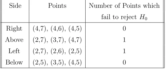
The largest rectangle where µ > δ within Pattern B holds the eight points where

i= 5,6,7,8 andj = 4,5. Suppose the initial point is in this set, (7,5). The

intersection-union test at first step in Region 1 tests the hypothesis on points (8,5) and (8,6). Both

points may be included in the rectangular set, but additional testing in Region 1 will

fail. The first step in Region 2 tests hypotheses at points (7,6) and (6,6). The test will

fail to reject H₀₁2 . Testing will not continue in Region 2. The first step in Region 3 will

test hypotheses at points (6,5) and (6,4). H3

01 will be rejected; (6,5) and (6,4) will be included in the rectangular set. Just like in Region 1, testing beyond step 1 will also

fail in Region 3. The first step in Region 4 tests hypotheses at points (7,4) and (8,4).

H4

01 will be rejected; (7,4) and (8,4) will be included in the rectangular set. Step 2 in Region 4 will fail to reject H₀₂4 so expansion in Region 4 is halted. The points in the set are {(7,5),(8,5),(8,6),(6,4),(6,5),(7,4),(8,4)}. With testing complete in all four regions, restrictions must be considered. Boundaries, from testing within each region,

are imposed on the rectangular set: from Region 1: i ≤ 8, from Region 2: j ≤ 5, from Region 3: 6 ≤ i and from Region 4: 4 ≤ j, such that 6 ≤ i ≤ 8 and 4 ≤ j ≤ 5. So, the actual reported rectangular set is{(7,5),(8,5),(6,4),(6,5),(7,4),(8,4)}, listed in the order in which points entered the set.

Suppose instead, testing occurred in the following order, with boundary restrictions

imposed during testing: Region 2, Region 1, Region 4, Region 3. Intuitively, testing in

(53)

from Region 2. However, testing first in Region 2 serves to set restrictions for subsequent

testing in Regions 1, 4 and 3. These restrictions are, in fact, benefits which improve the

testing algorithm.

Restrictions to set boundary values on i and j ensure that testing will not extend

to points outside the boundaries. In this way, restrictions, or boundaries, may limit

the number of points tested at each step within Regions (1, 4 and 3). When testing is

complete within all four regions, fewer points will have been tested, the rectangular set

will be complete and no trimming is required.

Testing in Region 2 first sets a boundary above, limiting tests to points with j ≤ 5 and ignoring points where j >5.

Testing in Region 1 would look at points (8,5) and (8,6), however, with limits

im-posed, only data for (8,5) is tested in H₀₁1 . Further testing fails in Region 1. The boundary to the right is i ≤10 which may seem redundant because there are no points wherei >10. At this point, the rectangular set consists of{(7,5),(8,5)}. The boundary to the right is revised to i≤8.

Testing in Region 4 would examine (7,4) and (8,4). The boundaries do not restrict

any points in H4

01. These points will be included in the rectangular set. At step 2 in Region 4, the points involved are {(6,3),(7,3),(8,3),(9,3)}. Again, the limits on j do not affect this test. The restrictions on i eliminate (9,3) from being tested. H₀₂4 fails

to be rejected, so a limit below is set. Test points must now satisfy 4≤ j. Points with

(54)

limitations on testing points are 4≤j ≤5 and i≤8.

Testing at the first step in Region 3 would include (6,5) and (6,4). H3

01 is rejected. At step 2, test points would include{(5,6),(5,5),(5,4),(5,3)}, however, with boundaries imposed, only two points, (5,5) and (5,4), satisfy the restrictions. So, H₀₂4 is rejected.

The hypothesis at step 3 will test {(4,7),(4,6),(4,5),(4,4),(4,3),(4,2)}. Four points are eliminated by boundaries; only (4,5) and (4,4) are tested. H4

03 is not rejected. After step 3 in Region 4, the final boundary, from the left, is added to the restrictions, 5 ≤i. Testing in Region 3 adds {(6,5),(6,4),(5,5),(5,4)}to the rectangular set.

At the conclusion of testing, the rectangular set is

{(7,5),(8,5),(7,4),(8,4),(6,5),(6,4),(5,5),(5,4)}

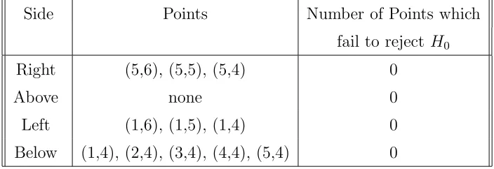
and the restrictions or boundaries 5≤i≤8 and 4≤j ≤5 have already been imposed. In Pattern C, suppose the initial point is (3,2). Using the algorithm from Section 2.2,

the rectangular set would include {(3,2),(4,2),(4,3),(3,3)}. This set is found by first testing (4,2) and (4,3) in Region 1 at step 1. Then, at step 2,{(5,1),(5,2),(5,3),(5,4)} are tested but not included in the rectangular set. In Region 2, (3,3) and (2,3) are

tested in step 1. Both points may be included in the rectangular set. In step 2,

{(2,4),(3,4),(4,4)} are tested but fail to be included. The first step in Region 3 tests (2,2) and (2,1). These points are not included in the rectangular set. Last, in Region 4,

step 1 tests (3,1) and (4,1), but neither are included in the rectangular set. Because of

(55)

Instead, suppose testing were ordered as follows, Region 3, Region 4, Region 1, Region

2. Testing in Region 3 would not add any points to the rectangular set, but would restrict

future testing to 3 ≤i. No points from Region 4 would be added, but testing would be further restricted by 2 ≤j. In Region 1, only (4,2) and (4,3) would be added. Further testing would be adjusted by restrictingi≤ 4. Finally, in Region 2, only (3,3) would be included in the rectangular set because 3 ≤ i. The j boundary is set at j ≤ 3. In this example, the same rectangular set was found, {(3,2),(4,2),(4,3),(3,3)}. Changing the order of testing yielded no worse results than the Original algorithm produced.

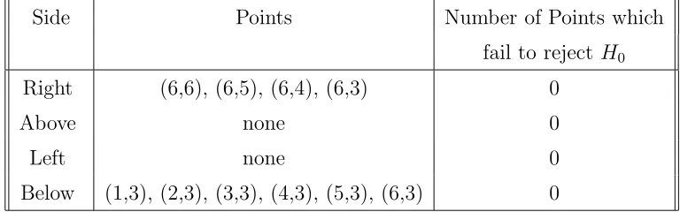
In Pattern D, the change in testing order can have a dramatic effect. Suppose (3,6) is

the initial point. The first step of testing in Region 1 would include points (4,6) and (4,7)

in the rectangular set. In the second step,H1

02tests{(5,5),(5,6),(5,7),(5,8)}and fails to be rejected. In Region 2, the first step of testing would examine data at (3,7) and (2,7).

H₀₁2 is not rejected so no points are added to the rectangular set. Data at points (2,6) and (2,5) are tested at the first step in Region 3. H3

01is rejected and these points are included in the rectangular set. The second step in Region 3 tests {(1,7),(1,6),(1,5),(1,4)}. H₀₂3

is not rejected. At the first step in Region 4, (3,5) and (4,5) are studied. H₀₁4 is rejected.

H4

02 tests {(2,4),(3,4),(4,4),(5,4)} and may include all these points in the rectangular set. H₀₃4 tests {(1,3),(2,3),(3,3),(4,3),(5,3),(6,3)} and may include all these points in the rectangular set. H₀₄4 tests {(1,2),(2,2),(3,2),(4,2),(5,2),(6,2)} and fails to be rejected. Testing in Region 4 includes the following points in the rectangular set