Symbolic formulation and diffusive resolution of
some operational problems:
theory and applications to optimal control
M. Lenczner
∗and G. Montseny
†January 20, 2006
2000 Mathematics Subject Classification: 47B34, 47G10, 49N05, 47A48, 93C20, 93B40 Keywords: Integral operators, Diffusive realization, Operational equation, Riccati equation, Lyapunov equation, Computational method
Abstract: This paper is focused on the derivation of state-realizations of diffusive type for linear operators solutions of some operatorial equations. We first establish two general theoret-ical framework fitted respectively for regular symbols and for symbols having their singularity located on the real axis. In a second part, we treat two Lyapunov equations issued from the stabilization theory for the heat equation. We also present an example that is beyond the linear framework introduced in this paper, namely a Riccati equation. The practical interest of this work relates to the context of intensive computation in embedded systems, in particular when embedded computers have Cellular Neural Networks-like architectures.
1
Introduction
Our concern when developing the method presented in this paper relates to embedded intensive computation based on networked computers. Potential applications are in many fields of physics where intensive calculations have to be made in real time with embedded computers for the treatment of arrays of data. Let us mention a few of them: detections of moving acoustic sources, control of acoustic noise, vibrations damping, control in fluid mechanics, measure of brain activity, radars, etc.In most of applications that require intensive embedded computations,
DSPs networks are employed. An alternative hardware solution is now emerging, the so-called 00Cellular Neural Networks00 (CNN) technology. The original idea appeared in the celebrated
pioneering paper of L. Chua [2]. Since this visionary work, much time and energy have been spent to develop this new technology that become more and more mature. Today-applications are mainly oriented towards image processing with a large spectrum of potential industrial
∗Center for Research in Scientific Computation, North Carolina State University, Raleigh, NC 27695. E-mail
address: [email protected].
application. However, we think that, in the next decade, we will assist to the emergence of a large variety of applications in many other fields.
A Cellular Neural Network is an array of interconnected analogic processors (see T. Roska and L. Chua [3] for details). Today0s available CNN0s chips have 128x128 analogic intercon-nected programmable cells. The basic operation (or instruction) in a CNN consists in solving a system of (non-linear) differential equations with as many variable as cells in the array and with programmable coefficients. These coefficients are spatially invariant and are so that they couple each cell with their closest neighbors. With such an architecture, realization of finite dif-ferences operator associated to one-dimensional or two-dimensional finite differences equations is an easy task. Additional basic instructions which produce local simple algebraic operations as additions or multiplications may also be available. A CNN can also execute a sequence of elementary instructions. Its input and output data are arrays of numbers. The huge ad-vantage of the CNN computers is that a basic instruction operates on a very large amount of data (128x128) in an extremely short time (a few nanoseconds). This is for example the time required for the resolution of the Laplace equation.
Here, we address the problem of the concrete realization of linear operators on infinite dimensional spaces in a way that be compatible with real time and embedded computation, possibly implantable on such CNNs, i.e. that requires only the few possible operations already mentioned.
Other authors have already studied the same kind of questions. B. Bamieh and its co-workers have developed in [1] a method that produces approximate realizations of operators. It furnishes, when it exists, an approximation under the form of a convolution product between the input and a kernel having a small support. Their method is limited to a class of space invariant operators, which excludes optimal control on bounded domains (in particular the case of boundary control or boundary observation). For the same class of problems, the authors have built in [4] optimal approximate realizations based on combination of finite differences operators. The coefficients of the approximate operator are obtained from numerical resolution of Linear Matrix Inequalities (LMIs), which have not always a solution. The authors announced that their method could be extended to bounded domains and also to boundary control or observation. In [5], the authors have built an approximation in the sense of high frequencies, by means of a cascade of partial differential equations. At the moment, this method is restricted to operational equations whose coefficients are all depending on the same partial differential operator. It turns out that it cannot handle with the kind of operators that we get in optimal control theory when observations or controls are on the boundary (or concentrated on some particular point in the domain). Let us stress out that both methods developed in [4] and in [5] suffer of some strong limitations that we aim to overcome in this paper.
(involving the resolvent of operator∂x in the algebra of causal linear bounded operators onL2):
P u(x) =
Z
µ(x,ξ)(∂x+θ(ξ)I)−1u(x)dξ; (1)
so the numerical realization ofP,approximated at any nodexi, requires the resolution of finite
differences equations,P ue (xi)≈Pnµ+n(xi)(∆x+θ(ξn)I)−1u(xi). This approach involves on the
one hand the Laplace transform P of the impulse response y 7→ Pδ(x−y) of the operator P
under consideration. It involves on the other hand a specific parameterized complex path θ
such that−θ1 is located in the intersection of the closure of the domain of holomorphy of
P and a half complex plane located to the left of a vertical line. If −θ does not touch any singularity of P, then the so-calledθ-symbol µis a regular function; otherwise it is a generalized function. General 1D-operators are decomposed in a causal and an anti-causal parts, and each of them admits a representation like (1).
The theory of diffusive representation and its applications have been broadly developed in [12] and the references therein. They have been reported in a recent monograph [8] in which a general framework is introduced and applications covering a large range of fields are presented. One of the main recognized advantages of the diffusive representation is the low computational cost of concrete realizations of integral operators derived from this approach (see for example [6]). Until now, a large part of the studies have been focused on one-dimensional problems where the operatorsP were given explicitly. However, we stress that in many cases, the theory can be extended to any dimension (see for example [8] where diffusive realizations of an nD-operator are introduced and applied to a problem of image processing).
This paper is the first attempt to build diffusive realizations of operators that are themselves the unknowns of operational equations. Our main contribution consists in the determination of the equations verified by µ and in the characterization of the admissible paths θ. Our intention is to provide a self-contained paper relating to the bases of this approach. For the sake of simplicity, the presentation is limited to regular µ in the general case and to possibly generalized functions in the simpler particular case whereθis a degenerated contour with empty interior, which is sufficient to broach many practical situations. In both cases, we prove the equivalence of the obtained equation onµ and the given operational one onP, and an explicit sufficient condition for existence of such a path θ is stated. Note that this work is concentrated on the mathematical formulation of the method only: practical aspects relating to specific applications, implementation, etc. are postponed to a further publication.
A substantial validation of this approach is provided through two examples of Lyapunov equations (issued from stabilization theory of the heat equation). In the case where the path
θ go through the singularities of P (which are here concentrated on the real axis), a suitable formal method based on the resolution of some auxiliary one-dimensional boundary value prob-lems allows the explicit analytical determination of µ. Finally, a non-linear Riccati equation associated to a boundary optimal control problem is treated formally. Through this example, it can be appreciated that the treatment of boundary controls (the same thing holds for boundary observations) can be handled, in principle, by this method.
1The path
The paper is organized as follows. The framework of diffusive representation and state realizations of integral operators is presented in section 2. In section 3, we state and prove the main results relating to symbolic equation satisfied by the diffusive symbols and equivalent to the operational equation under consideration. Finally, the sections 4, 5 and 6 are focused on the treatment of concrete examples.
2
Di
ff
usive realization of integral operators
Our intention is to provide a self-content paper in a necessarily simplified framework but nev-ertheless applicable to a large class of practical situations. So we limit our presentation to two classes of operators and paths. The first one refers to paths that lie far from the singularities of the Laplace transformP, so the diffusive symbols are regular. The second one is a special case of paths crossing some singularities, namely the case where they and all the singularities belong to the real axis. Such paths go necessarily through all singularities and therefore the diffusive symbols are some generalized functions. In both cases, we state and prove the existence of diffusive realizations and symbols and we discuss the question of uniqueness.
We consider bounded operatorsP in L2(ω) formulated under the general integral form
P u(x) =
Z
ω
p(x, y)u(y) dy
where ω=]0,1[and where the kernel p(x, y)has a regularity specified later2.
2.1
Definition and general properties
An operatorP is said to be causal (respectively anti-causal) ifp(x, y) = 0fory > x(respectively for y < x). Diffusive realizations ofP are based on its (unique) decomposition into causal and anti-causal parts,
P =P++P−,
where
P+u(x) =
Z x
0
p(x, y)u(y)dy and P−u(x) =
Z 1
x
p(x, y)u(y)dy.
Throughout this paper, we shall use the uperscripts + or − to refer to causal or anti-causal operators, and the convention ∓=−(±).
The so-called impulse responsepeis defined from the kernel p(x, y)by
p(x, y) =pe(x, x−y)with (x, y)∈Ω
2Note that for the applications we have in mind, unbounded operators may occur; in such a case, they can
or conversely by
e
p(x, y) =p(x, x−y) with (x, x−y)∈Ω
where Ω=ω×ω. The variablesx andy are treated on an unequal footing, assuming that the causal (resp. anti-causal) impulse response is analytic with respect toy, with locally integrable analytic extension to R+∗ (resp. R−∗) and that for each frozeny, x7→p(x, y)∈L2(ω).
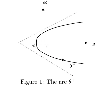
For givena± ∈R,let us considerξ7→θ±(ξ)two complex continuous and almost everywhere differentiable functions from Rto[a±,+∞[+iR,a ∈R, with derivativesθ±0 such that0<α≤ |θ±0|≤β <+∞, and which define two simple oriented arcs closed at infinity. We also suppose, for various reasons not recalled here (see [12]), thatθ± are located inside a sector defined by two non vertical straight lines as shown in Fig 1. Note that this last condition implies that equation (51) is of diffusive nature (see [11]); this justifies the terminology 00diffusive representation00.
θ +
0 R
iR
-a
Figure 1: The arcθ+
Remark 1 The approach presented hereafter may also be formulated with bounded arcs θ±
parameterized on R/2πR≡[0,2π[ instead of R, so that θ± are closed contour. Up to minor technical adaptations, all the results of this section remain valid after changing R by [0,2π[.
From now on, we use the convenient notation:
hµ,ψi:=
Z
R
µ(ξ)ψ(ξ)dξ; (2)
note that in the case whereµwould not be a locally integrable function, a more general duality product, to be specified in each concrete case3, would be involved in place of the integral.
De&nition 2 (i) A causal operator P+ (resp. anti-causal operator P−) admits a diffusive
θ+-realization (resp. θ−-realization) if there exists a so-called diffusive symbol4 µ+(x,ξ) (resp.
µ−(x,ξ)) so that
P+u(x) =µ+,ψ+(u)® (resp. P−u(x) = µ−,ψ−(u)®), (3)
where ψ±, the so-called θ±-representations of u, are defined by
ψ+(u)(x,ξ) =
Z x
0
e−θ+(ξ)(x−y)u(y) dy and ψ−(u)(x,ξ) =−
Z 1
x
eθ−(ξ)(x−y)u(y) dy ∀ξ∈R+. (4)
(ii) An operator P admits aθ±−diffusive realization if both its causal and anti-causal parts
P+ and P− admit a diffusive realization associated respectively to θ+ and θ−.
Note that in (4), u can be taken in the space of measures without loss of regularity of ψ; therefore, the causal part of the impulse response can be writtenpe(y) =Dµ, e−θ+(ξ)yEand it
re-sults that Fubini theorem is valid: R0xDµ, e−θ+(ξ) (x−y)E u(y)dy =Dµ,R0x e−θ+(ξ) (x−y)u(y)dyE. The same thing can be done for the anti-causal part.
The functions ψ±(u) can be characterized as the unique solutions of the following direct and backward Cauchy problems, parameterized byξ ∈R:
∂xψ+(x,ξ) =−θ+(ξ)ψ+(x,ξ) +u(x)∀x∈]0,1[, ψ+(0,ξ) = 0 (5)
and ∂xψ−(x,ξ) =θ−(ξ)ψ−(x,ξ) +u(x)∀x∈]0,1[, ψ−(1,ξ) = 0, (6)
which constitute together with (4) a diffusive state-space realizations ofP+andP−respectively. This last point is central in view of concrete approximated realizations ofP. The proposition 5 in subsection 2.2 shows that the half ofθ±can be sufficient for the realization of real operators. The following proposition state that self-adjoint operators can be expressed with respect to
µ+orµ−only. This property will be useful for instance in the treatment of non-linear equations such as Riccati ones, where the equations of µ+ andµ− are not directly discoupled.
Proposition 3 If there exists a diffusive realization of a self-adjoint operator P, then it may be realized with only one of the two symbols µ+ or µ− :
P u(x) = µ+(x,ξ),ψ+(u)(x,ξ)®+
Z 1
x
D
µ+(y,ξ), e−θ+(ξ)(y−x)E u(y) dy
and P u(x) = −
Z x
0 D
µ−(y,ξ), eθ−(ξ)(y−x)Eu(y) dy−µ−(x,ξ),ψ−(u)(x,ξ)®
from which is deduced the relation between the causal and anti-causal parts of the kernel and the diffusive symbols,
p(x, y) =Dµ+(x,ξ), e−θ+(ξ)(x−y)E=−Dµ−(y,ξ), eθ−(ξ)(y−x)E for y ≤x
and p(x, y) =−Dµ−(x,ξ), eθ−(ξ)(x−y)E=Dµ+(y,ξ), e−θ+(ξ)(y−x)E= for y≥x.
Proof. According to the expression of diffusive realization ofP+ andP−, one deduces the relation betweenp(x, y) andµ±,
p(x, y) =Dµ+(x,ξ), e−θ+(ξ)(x−y)E fory ≤xandp(x, y) = −Dµ−(x,ξ), eθ−(ξ)(x−y)E forx≤y.
Now, the symmetry of p(x, y) =p(y, x) yields an expression of
P−u(x) =
Z 1
x
p(y, x)u(y)dy
with a kernel p(y, x) for x < y that may be formulated as a function of µ+ so that the first formula for P u follows. The second one is obtained by using a similar argument that leads to an expression of P+uwith respect to µ−.
2.2
Canonical (regular) di
ff
usive realization
In this section we state some sufficient conditions for the existence of the so-called canonical diffusive realization of an operator P for general paths θ±. Its proof is constructive starting from the impulse response. The conditions for existence pertain to the Laplace transforms5
with respect to y,P+(x,λ) =
Ly(pe(x, y))(λ) andP−(x,λ) =Ly(pe(x,−y))(λ) of the causal and
anti-causal parts of the impulse response.
Theorem 4 For a given path θ+ (resp. θ−), a causal (resp. anti-causal) operator P+ (resp.
P−) admits a diffusive symbol if the two following conditions are fulfilled:
(i) the Laplace transform λ7→ P+(x,λ) (resp. λ 7→P−(x,λ)) is holomorphic in a domain
D+ (resp. D−) that contains the closed set located at right of the arc −θ+ (resp.
−θ−); (ii) P±(x,λ) vanish when |λ|→ ∞ uniformly with respect to argλ.
Then the so-called canonical θ±-symbols are given by
µ+(x,ξ) = θ
+0(ξ)
2iπ P
+
(x,−θ+(ξ)) and µ−(x,ξ) = −θ
−0(ξ)
2iπ P
−(x,
−θ−(ξ)) (8)
and have the same regularity as θ±0.
Proof. The Laplace transformP+ is holomorphic on the right of a vertical line, Re(z) ≥a
then pe(x, y) can be expressed, thanks to the inverseL−1 of the Laplace transform, by
e
p(x, y) =L−1(P+(x,λ))(y) = 1 2iπ
Z
a+iRP +
(x,λ)eλydλ. (9)
Since P+ is assumed to be holomorphic at the right of
−θ+ and to vanish uniformly at infinity, the Jordan lemma and the Cauchy theorem allow to prove thatpe(x, y) =−21iπR−θ+P+(x,λ)eλy
dλ = −21iπR−θ+P+(x,λ)eλy dλ =
R R
θ+0(ξ)
2iπ P
+(x,
−θ+(ξ))e−θ+(ξ)y dξ. This completes the proof
of existence fromP+u(x) =Rx
0 pe(x, x−y)u(y) dy and from the expression (4) of ψ +
. The proof is similar for the anti-causal part, considering withpe(x,−y)when y <0.
When it exists, the canonical diffusive realization of an operator is necessarily unique, but an infinity of (non-canonical) diffusive realizations exists also. This can be seen by inspection of the kernel of the linear operators
µ± 7→µ±,ψ±(u)®,
5Note that
P±are the so-called symbols, in the sense of Laplace Transform, of operatorsP±which therefore are frequently denotedP±(x,±∂
which includes any function ξ 7→ µ±(.,ξ) defined by (3) with P+ (resp.
P−) holomorphic in the closure of the domain at left of θ+ (resp. at right of θ−).
The next proposition shows that the half θ± can be sufficient for the realization of real valued operators or equivalently real valued impulse responses.
Proposition 5 If P is real valued and if the paths θ± are symmetric with respect to the real axis, that is θ±(−ξ) =θ±(ξ) then µ±(−ξ) =µ±(ξ) and
µ±,ψ±®= 2 Re
Z +∞
0
µ±ψ±dξ
so that the the diffusive realization can be parameterized on a half path θ±∗ =θ±|R+.
Proof. If θ±(−ξ) =θ±(ξ) then ψ±(x,−ξ) =ψ±(x,ξ). Since P is real valued it comes that P±(x,λ) =P±(x,λ)and therefore µ±(−ξ) =µ±(ξ). We therefore have:
µ±,ψ±®=
Z +∞
0
µ±ψ±dξ+
Z 0
−∞
µ±ψ±dξ=
Z +∞
0
µ±(x,ξ)ψ±(x,ξ) +µ±(x,−ξ)ψ±(x,ξ)dξ.
So µ±(−ξ) =µ±(ξ) yields
µ±,ψ±® = 2 Re
Z +∞
0
µ±ψ±dξ.
Remark 6 It is useful to draw attention to the fact that the causal (resp. anti-causal) part of the impulse response is necessarily analytic on R+∗ (resp. R−∗) and locally integrable on R+ (resp. R−) with respect to the second variable y. As a matter of fact, this can be observed, for instance, on the causal part. The expression of pe+(x, y) =R
R
θ+0(ξ)
2iπ P
+(x,
−θ+(ξ))e−θ+(ξ)y dξ
may be extended to complex numbers y belonging to a vicinity of R+ thanks to hypothesis on
θ+; such a function being also derivable, it is analytic.
2.3
On some singular di
ff
usive realizations
In the theorem 4 we have assumed that the paths θ± do not intersect with the singularities of the Laplace transforms P±. A similar result has been established under weaker hypothesis in [8], including the case whereP± may have singularities on the arcsθ±.This result have already found some interesting applications [12]. The general proof is more technical: it necessitates to consider Rθ in the sense of finite parts and from the topological viewpoint, it involves fitted Fréchet spaces ∆θ± 3 ψ(x, .) with topological dual ∆0θ± 3 µ(x, .). Let us mention that in
such a case, the diffusive symbols µ± are some generalized functions. For this reason, the corresponding diffusive realizations will be called singular diffusive realizations.
Let us start by a general remark on diffusive realization with closed paths θ± having an empty interior. They may be parameterized on a symmetric way so that θ±(−ξ) = θ±(ξ),
ψ±(−ξ) =ψ±(ξ)and therefore
µ±,ψ±®=
Z +∞
0
µ±(x,ξ)ψ±(x,ξ)dξ+
Z 0
−∞
µ±(x,ξ)ψ±(x,ξ)dξ
=
Z +∞
0
(µ±(x,ξ) +µ±(x,−ξ))ψ±(x,ξ)dξ.
Posing µ±∗(x,ξ) = µ±(x,ξ) + µ±(x,−ξ) yields to a diffusive realization on the half paths
θ±∗ =θ±|R+ (parameterized onR+ only) formally expressed by:
=
Z +∞
0
µ±∗(x,ξ)ψ±(x,ξ)dξ;
more rigorously, since µ±∗ can be a generalized function, this will be preferably denoted by
µ±∗,ψ±®without possible confusion with the previous notation. An important particular case is when θ±∗ are some straight half lines: θ±∗(ξ) = ±λ0 ±σξ, λ0 and σ being some complex numbers; then:
e
p(x, y) =e−λ0y(
Lµ+∗(x, .))(σy)and pe(x,−y) =−e+λ0y(
Lµ−∗(x, .))(σy) for y∈R+, (10)
where L is the Laplace transform defined in the set D0
+ of distributions with support in R+. As we consider here real operators (and so impulse responses) only, the singularities ofP± are necessarily conjugate. So they are necessarily concentrated on a half straight line included in the real axis. In the following, we will assume that λ0,σ ∈ R. The next proposition states existence and uniqueness of a such a singular diffusive realization.
Proposition 7 An operator P has a θ±∗-diffusive realization with unique symbols µ±∗ ∈ D0 + iff for all x ∈ ω the causal and anti-causal parts of the impulse response p˜(x, .) are locally integrable with analytic continuation holomorphic in R±∗+iR and there exists some constants
c± so thatp˜(x,±y)e±λ0y are bounded uniformly inx by some polynomial functions of|y| for all
y such thatRey > c±.
Proof. This statement comes directly from the characterization of the range of the Laplace transform established by L. Schwartz, see e.g. [9].
3
Di
ff
usive symbolic formulation of linear operational
equations
More precisely, we will state the equations satisfied by the diffusive symbols µ± equivalent to a boundary value problem posed on the kernel p in Ω+
∪Ω− where Ω± correspond to the causal (y < x) and anti-causal(y > x)parts of Ω. For this purpose we make a partition of the boundary of Ω± in Γ+
y ={1} ×ω, Γy− ={0} ×ω, Γ0 = {(x, y) ∈Ω s.t. x =y}, Γ+x =ω× {0}
and Γ+x =ω× {1}. We establish the results successively for the canonical θ±-symbols µ± and
then for the singular θ±∗-symbols when θ±⊂R.
3.1
Canonical formulations
Let us start by stating the equations satisfied by diffusive symbols associated to a kernel p
solution of a partial differential equation (the boundary conditions will be taken into account later):
A(x, y,∇)p(x, y) =q(x, y) (11)
where we denote ∇ = t(∂
x,∂y) and q is the kernel of a given operator Q. With φ±(x, y) =
(x,±(x−y)), the partial differential equation solved by ep± =p◦φ±, is e
A±(x, y,∇)pe± =qe± (12)
where Ae±(x, y,∇) =A(φ±(x, y), K±∇) andK± = µ
1 ±1 0 ∓1
¶
.
Recall thatpe± has analytic continuation onR+∗; we assume that this is also the case for Ae (with respect to y). Furthermore, we can extendAe± andpe± toR− by0; so, the formulation of (12) in the sense of distributions takes the form:
e
A±(x, y,∇)ep±+X
k
e
A±k(x,∇)pe± δ0(k) =eq± inD0+(R), (13)
where Ae±k(x,∇) are suitable partial differential operators and δ(0k) is the kth derivative of the
Dirac distribution at0.We are now in position to introduce two differential operators associated to A andθ±:
A±(x, y,∂x,λ) =A(x, y, K±(∂x,−λ))
A±0(x,∇,θ±(ξ)) =±θ
±0
(ξ) 2iπ
X
k
(−θ±(ξ))kAe±k(x, K±∇)
and the weight c(λ) = (λ+λ±0)−n, for a λ±
0 ∈C−D± and n being the lowest positive integer so that c(λ) maxk|λkAek(x,η,λ)| vanishes when |λ| tends to infinity for allη. The first lemma
is related to the case where the partial differential equation (11) is satisfied for a given value of x and for y belonging to an open interval ω0 that is partitioned in ω0+ = ω0∩]− ∞, x] and
ω−0 =ω0∩[x,+∞[.
y∈ω±0
D
c(θ±(ξ))[A±(x, y,∂x,θ±(ξ))µ±(x,ξ) +A±0(x,∇,θ±(ξ))p(x, x)], e−
θ±(ξ)(x−y)E=c(∂
y)q(x, y).
(14)
If in addition the coefficients of A are independent of y and Q admits a θ±−diffusive re-alization with canonical symbols ν± then the integral equation (14) is equivalent to the local formulation for all (x,ξ)∈ω±0 ×R+
A±(x,∂x,θ+(ξ))µ±(x,ξ) +A±0(x,∇,θ±(ξ))p(x, x) =ν±(x,ξ). (15)
Remark 9 The termp(x, x) can also be replaced by hµ±(x, .),1i.
Proof. We detail only the causal case and remove some indexes+ for the sake of simplicity. The anti-causal case follows exactly the same steps with pe− in place of pe+.
We use the same notations that in theorem 4,P+and
Q+denoting the Laplace transform of the causal parts of the impulse responsespeandqeanalytically extended to R+∗. From (13) and ∇ep =∇L−1Lep =
L−1((∂
x,λ)P+(x,λ)), we deduce that Ae(x, y,∇)L−1L(pe) +PkAe+k(x, y,∇)pe
δ(0k)=qeor equivalently that P+ solves
L−1(Ae(x, y,∂x,λ)P+(x,λ) +
X
k
h e
A+k(x,∇)pei(x,0)λk) =q.e
Furthermore, ifQhas a diffusive realization thenqe=q◦φ =L−1Q+ and if the coefficients of A are independent of y, thanks to the injectivity of the inverse Fourier-Laplace transform L−1 and to the definition of Ae(x,t(∂
x,λ)) =A+(x, K t(∂x,λ)), we get
A+(x, K(∂x,λ))P+(x,λ) +
X
k
λkhAe+k(x,∇)pei(x,0) = Q+(x,λ)
which holds for all λ in the domain of holomorphy of P+ and
Q+ and in particular for λ = −θ+(ξ).Taking into account the definition of the canonical symbolsµ+(x,ξ) = θ+0(ξ)
2iπ P
+(x,
−θ+(ξ))
and ν+(x,ξ) = θ+
0
(ξ) 2iπ Q
+(x,
−θ+(ξ)), posing λ = −θ+(ξ) and using the relation ∇ep(x,0) =
K±∇p(x, x) we get (15).
In the general case of coefficients depending on y, we argue as in the theorem 4. But this cannot be done directly because the functions λ 7→ λk
h e
A+k(x,∂x,λ)pe
i
(x,0) in general do not vanish at infinity. So we introduce the weightc(λ)so thatc(λ)λkAe+k(x,∂x,λ)vanishes at infinity
and we remark that:
L−1 h
λkAe+k(x,∂x,λ)pe
i
(x,0) =c(−∂y)−1L−1
h
c(−λ)λkAe+k(x,∇)pe i
(x,0) inD+0 .
Sincec(−∂y)−1 is injective (as operator inD+0 ) andA+(φ(x, y),∂x,−λ) =Ae(x, y,∂x,λ)it comes
L−1(c(−λ)[A+(φ−1(x, y),∂x,−λ)P+(x,λ) +
X
k
Using the same argument than in the theorem 4, this is equivalent to D
c(θ+(ξ))[A+(φ−1(x, y),∂x,θ+(ξ))µ+(x,ξ) +A+0(x,
t
∇,θ+(ξ))p(x, x)], e−θ+(ξ)yE
=c(−∂y)qe(x, y).
The final formulation is in the original domain Ω+ : D
c(θ+(ξ))[A+(x, y,∂x)µ+(x,ξ) +A+0(x,t∇,θ +
(ξ))p(x, x)], e−θ+(ξ)(x−y)E=c(∂y)q(x, y)
because (−∂y)(q◦φ)(x, y) = (∂yq)◦φ(x, y).
The second lemma refers to the case where the equation (11) is a constraint that must be satisfied on an isolated value of y, useful for taking into account boundary conditions (its formulation in term of symbols is not specific to regular θ±-symbols and will also be applied to singular symbols).
Lemma 10 Let us assume that P fulfils the assumptions of theorem 4. The kernel p satisfies (11) for a given couple (x, y) iff the symbols µ± verifies
D
A±(x, y,∂x,θ±(ξ))µ±(x,ξ), e−θ
±(ξ)(x−y)E
=q(x, y). (16)
Proof. We make the proof in the causal case only and omit some indexes+. Since
A(x, y, K∇)ep◦φ−1 =q (17)
and from the relationpe(x, y) =
D
µ+(x,ξ), e−θ+(ξ)y
E
on the causal domain:
A(x, y, K∇)Dµ+(x,ξ), e−θ+(ξ)yE◦φ−1 =q
thus
D
A(x, y, K¡∂x,−θ+(ξ)
¢
)µ+(x,ξ), e−θ+(ξ)(x−y)E=q(x, y)
or equivalently
D
A+(x, y,∂x,θ+(ξ))µ+(x,ξ), e−θ +(ξ)(x
−y)E=q(x, y) (18)
that leads immediately to the announced result.
Consider now a boundary value problem posed on the kernelp:
A(x, y,∇)p(x, y) = q(x, y)in Ω+∪Ω− (19)
with an unspecified number of boundary conditions
Operators B± andB±
0 can be derived from B on the same manner that A± and A±0 was from
A. The counterpart of equations (14), (15) and (16) are the integral equation onΓ±
y:
D
c(θ±(ξ))[B±(x, y,∂x,θ±(ξ))µ±(x,ξ) +B0±(x,∇,θ±(ξ))p(x, x)], e−
θ±(ξ)(x−y)E=c(∂
y)r(x, y),
(21)
its local formulation
B±(x,∂x,θ+(ξ))µ±(x,ξ) +B0±(x,∇,θ±(ξ))p(x, x) =ρ±(x,ξ) onΓ±y and∀ξ∈R
+
(22)
and finally the integral equation related on Γ±
x ∪Γ0
D
B±(x, y0(x),∂x,θ±(ξ))µ±(x,ξ), e−θ
±(ξ)(x−y0(x))E
=r(x, y0(x)) (23)
with y0(x) = x, 0 or 1 on Γ0, Γ+ or Γ−. The restrictions of r to the boundaries Γ±y are the
kernels of a causal operator R+ and an anti-causal operator R−. When they have a diffusive realization their symbols are denoted by ρ+ andρ−.
Theorem 11 Assuming that P fulfils the assumptions of theorem 4,
(i) its kernel is solution of the boundary value problem (19-20) iff its canonical θ±−symbols are solution of (14) on Ω±, (21) on Γ±
y and (23) on Γ±x ∪Γ0;
(ii) if in addition the coefficients of A and B are independent ofy and the operators Q, R± fulfils the assumptions of theorem 4 then the integral equations (14) and (21) are equivalent to their local formulations (15) and (22).
For ending the section we establish some sufficient conditions on the operators A and B,
with coefficients independent ofy,that insure that P satisfies the assumption (i) of theorem 4. The differential operators A± andB± can be expanded with respect to the derivatives:
A±(x,∂x,λ) =
X
m
a±m(x,−λ)∂xm andB±(x,∂x,λ) =
X
m
b±m(x,−λ)∂xm,
which allows to define the union of zeros of the analytic functions λ 7→ a±
m(x,−λ) and λ 7→
b±m(x,−λ)over all x andm:
WA± :=[
x,m
[a±m(x, .)]−1(0)andWB± :=[
x,m
[b±m(x, .)]−1(0). (24)
Theorem 12 IfWA±∪WB± ⊂C−D± and if Q andR± fulfil the assumption (i) of the theorem 4 then P fulfils it also.
3.2
Formulation in some singular cases
In this section, we establish the counterpart of theorem 11 in the particular framework of singular diffusive realizations introduced in the section 2.3, whenθ±(ξ) = ±λ0+|ξ|,θ±∗ =θ±|R+.
Lemma 13 Let us assume that P admits a θ±∗-diffusive realization, that the coefficients of A
are independent of y and that Q admits a θ±∗-diffusive realization; then p is solution of (11) for all x, y∈ω0 iff
A±(x,∂x,θ±(ξ))µ±(x,ξ) =ν±(x,ξ) for all x∈ω±0.
Proof. The proof is for the causal case only. Since equation (11) holds for all y∈ ω+0 and
A is independent of y, the equation (17) is equivalent to
A(x, Kt∇)pe(x, y) = qe(x, y) for y∈ω+0. (25)
From proposition 7 analytic continuation of (25) holds for all complex numbers y ∈R+∗+iR.
Thus
L(A+(x,∂x,θ+(ξ)µ+(x,ξ)−ν+(x,ξ))(y) = 0 for all y∈R+∗+iR.
Thanks to injectivity of the Laplace transform, this is equivalent to
A+(x,∂x,θ+(ξ)µ+(x,ξ) =ν+(x,ξ).
The subsequent equations satisfied by the symbols are derived directly from the lemmas 10 and 13.
Theorem 14 Assume that P has a θ±∗−diffusive realization.
(i) The kernel p is solution of the boundary value problem (19-20) iff
D
A±(x, y,∂x,θ±(ξ))µ±(x,ξ), e−θ
±(ξ)(x−y)E
= q(x, y) in Ω± (26) D
B±(x, y,∂x,θ±(ξ))µ±(x,ξ), e−θ
±(ξ)(x−y)E
= r(x, y) on Γ0∪Γ±x ∪Γ±y.
(ii) If the coefficients ofAandB are independent ofyand if QandR±have someθ±∗−diffusive realizations then the integral equations (261) and the restriction of (262) to Γ±
y are equivalent
to the local equations
A±(x,∂x,θ±)µ±(x,ξ) = ν±(x,ξ) in Ω± (27)
4
A Lyapunov equation with Dirichlet conditions
The results of this section will afford an illustration of theorem 11 for canonical symbols and of theorem 14 for singular ones. All the operators considered in the subsequent examples which admit a θ±−diffusive realization have also aθ±∗−diffusive realization in the sense of the proposition 5. In addition we will alway choose θ+∗ = θ−∗ in such a way that in all following we can simplify the notations by replacing θ±∗ byθ andD± byD.
In this section we study the diffusive symbol of the operator P solution of a Lyapunov equation that appears in the context of the internal stabilization of a system governed by the heat equation with Dirichlet boundary conditions. Let us consider a half pathθ, a non-negative constant cand Qa self-adjoint positive operator. The Lyapunov equation
Z
ω∇
u∇(P v) +∇(P u)∇v dx=
Z
ω
Qu v+cu v dxfor all u, v ∈H01(Ω), (28)
is well-posed in the set of operators P continuous from H01(Ω) to H01(Ω). Let us start by choosingc= 0and applying the theorem ??related to canonical symbols.
Proposition 15 Assuming that 06∈D, there exists a diffusive realization of P with canonical symbols µ± solutions of the discoupled set of equations:
(∂2xx−2θ(ξ)∂x+ 2θ2(ξ))µ+(x,ξ) + 2(∂xp(x,0) +∂yp(x,0))δ0(y) + 2p(x,0)δ00(y)
=ν+(x,ξ) ∀(x,ξ)∈ω×R+,
(∂x−2θ(ξ))µ+(x,ξ),1
®
= 0, µ+(x,ξ), e−θ(ξ)x®= 0 ∀x∈ω, (29)
µ+(1,ξ) = 0 ∀ξ ∈R+,
and
(∂xx2 + 2θ(ξ)∂x+ 2θ2(ξ))µ−(x,ξ) + 2(−∂xp(x,0) +∂yp(x,0))δ0(y) + 2p(x,0)δ00(y)
=ν−(x,ξ) ∀(x,ξ)∈ω×R+,
(∂x+ 2θ(ξ))µ−(x,ξ),1
®
= 0, µ−(x,ξ), eθ(ξ)(x−1)®= 0 ∀x∈ω, (30)
µ−(0,ξ) = 0 ∀ξ ∈R+.
Proof. The derivation of the boundary value problems satisfied by the causal and anti-causal parts of the kernel p of P is postponed after this proof. When c = 0, p is the unique solution of
−∆p(x, y) = q(x, y)on Ω andp(x, y) = 0 on ∂Ω. (31) Decomposingq(x, y) =P∞k,l=1qklsin(kπx) sin(lπy)on the orthogonal eigenvectors of the Laplace
operator with Dirichlet conditions, one easily deduces the expression ofpand therefore the ex-pression of the Laplace transforms P± which is seen to vanish when |λ| tends to infinity.
Now, let us turn to the derivation of the equation fulfilled by µ±. It is proved in the subsequent lemma that for all c ≥0 the causal and anti-causal parts of p are solutions of the two independent boundary value problems posed on Ω+ andΩ−
−∆p(x, y) = q(x, y) inΩ+, (32)
(−∂x+∂y)p|Ω+(x, y) =
c
2 onΓ0, p(x, y) = 0 on∂Ω
and
−∆p(x, y) = q(x, y) inΩ−, (33)
(−∂x+∂y)p|Ω−(x, y) = −
c
2 onΓ0 andp(x, y) = 0 on∂Ω
−−Γ 0.
According to the theorem 12 we find on the one hand the equations (29) and (30) and on the other hand that W±
a ={0} and Wb± = ∅. Then, existence of µ± is just a consequence of
existence of the kernel p.
Now, let us establish the boundary value problems satisfied by the kernel p.
Lemma 16 For anyc≥0, the causal and anti-causal parts of the kernelp ofP are the unique solutions of the two discoupled boundary value problems (32) and (33). In the particular case
c= 0, p is the unique solution of (31).
Proof. Plugging the kernel representation
P u(x) =
Z
ω
p(x, y)u(y) dy,
of P in the Lyapunov equation leads to ZZ
Ω
∂xu(x)∂x(p(x, y)v(y)) +∂x(p(x, y)u(y))∂xv(x)dy dx
=
Z
ω
c u(x) v(x) dx+
ZZ
Ω
q(x, y)w(x, y) dy dx,
or equivalently, due to the symmetryp(x, y) = p(y, x),
ZZ
Ω∇
p(x, y)∇w(x, y)dy dx = √1
2
Z
Γ0
c u(x)v(y)ds(x, y) +
ZZ
Ω
q(x, y)w(x, y) dy dx,
where w(x, y) = u(x)v(y)∈ H01(Ω) and Γ0 = {(x, y) ∈ Ω / x = y}. Since the set of functions
w(x, y) = u(x)v(y) with u, v ∈ H1
0(ω) is dense inH01(Ω) and p∈ H01(Ω) because the range of
P is assumed to beH01(Ω),we are in presence of a variational formulation on the form
p∈V, a(p, w) =l(w) for allw∈V
which fulfils the assumptions of the Lax-Milgram lemma, and therefore admits a unique solution
p∈H1
0(Ω). Whenc vanishes, this may be interpreted as (31).
When c6= 0, due to the presence of Dirac distribution in the right hand side, the solution cannot be found inH2(Ω)but only inH2(Ω+∪Ω−).So the strong form is written on each side of Γ0. Applying the Green formula in Ω−Γ0 =Ω+∪Ω− :
ZZ
Ω+∪Ω−−
(∆p+q)(x, y)w(x, y) dy dx+
Z
Γ0
1
√
2(−∂x+∂y)(p(x, y)|Ω+ −p(x, y)|Ω−)w(x, y) ds(x, y) = √c
2
Z
Γ0
which yields the strong formulation
−∆p(x, y) = q(x, y) onΩ+∪Ω−,
(−∂x+∂y)(p(x, y)|Ω+−p(x, y)|Ω−) = c onΓ0 andp(x, y) = 0 on∂Ω. Since p is symmetric, the second relation is equivalent to one of the two conditions
(−∂x+∂y)p(x, y)|Ω+ =
c
2 or(−∂x+∂y)p(x, y)|Ω− =−
c
2,
which ends the proof.
Now we examine the singular case whereθ =R+
⊃ −W ={0}and we apply the theorem 14.
The equations established in the previous proposition still hold excepted (291) that is replaced by
(∂xx2 −2θ(ξ)∂x+ 2θ2(ξ))µ+(x,ξ) =ν+(x,ξ).
As mentioned before, in such a case the diffusive symbols cannot be functions, and a suitable duality has to be chosen. We do not develop a complete theory for the equations of µ± in such a singular case, but we give their solutions in a particular case and propose a formal method that allows their derivation. The formal method consists in searching solutions µ± as the sum of a regular part g± and of an expansion of Dirac masses and their derivatives concentrated in
W ∩ −θ. In the current case, we search a solution on the form
µ+(x,ξ) =g+(x,ξ) +
n0
X
n=0
gn+(x)δ
(n)
(ξ) (34)
where n0 is assumed to be a finite, a priori unknown, positive integer.
Proposition 17 If Q = 0 and θ(ξ) = ξ, then P admits a diffusive realization with singular symbols
µ+(x,ξ) =g+0(x)δ(ξ) +g1+(x)δ0(ξ) and µ−(x,ξ) =µ+(1−x,ξ) ∀(x,ξ)∈ω×R+, (35) where g0+ and g1+ are the unique solutions of the two coupled boundary value problems
g0+00(x) + 2g+10(x) = 0 and g1+00(x) = 0 for all x∈ω (36)
g0+(0) = 0, g +
0(1) = 0, g +
1 (0) =−
c
2and g
+
1(1) = 0 their analytic expressions are
g+0 = x(12−x) and g1+ = x−21.
Proof. For the sake of clarity, we make the proof for c = 1. First, we state the relation between µ+ and µ−. Here, P is symmetric with respect to the center 1
2 of the interval, in the sense that
Then,
p(x, y) =p(1−x,1−y), pe(x, y) = pe(x−y,−y)andµ−(1−x,ξ) =µ+(x,ξ) ∀x∈ω.
Now, we suggest to use the more adequate boundary value problem which is equivalent to (29):
(∂xx2 −2θ(ξ)∂x+ 2θ2(ξ))µ+(x,ξ) = 0 ∀(x,ξ)∈ω×R+,
θ2(ξ)µ+(x,ξ),1®= 0 ∀x∈ω, (∂x−2θ(ξ))µ+(0,ξ),1
®
=−1
2,
θ2(ξ)µ+(x,ξ), e−θ(ξ)x®= 0 ∀x∈ω, µ+(0,ξ),1®= 0, (∂x−θ(ξ))µ+(0,ξ),1
®
= 0,
andµ+(1,ξ) = 0 ∀ξ ∈R+.
For its derivation, we differentiate the second equation in (29) with respect tox:
(∂xx2 −2θ(ξ)∂x)µ+(x,ξ),1
®
= 0,
and take into account (291) so that to deduce
−2θ2(ξ)µ+(x,ξ),1® = 0.
Associated with a boundary condition in 0,for example h(∂x−2θ(ξ))µ+(0,ξ),1i =−12, this is
equivalent to (292). The same procedure is applied to (293), with two derivations with respect to x. This yields
−θ2(ξ)µ+(x,ξ), e−θ(ξ)x® = 0,
and two initial conditions in x= 0,
µ+(0,ξ),1® = 0 and (∂x−θ(ξ))µ+(0,ξ),1
®
= 0.
Now that these equations are established, let us look for a solution on the form (34). From lemma 18, g+ and(g
n)0≤n≤n0 are solution of
(∂xx2 −2ξ∂x+ 2ξ2)g+(x,ξ) = 0, ∂xx2 g+0(x) + 2(∂xg1+(x) + 2g2+(x)) = 0,
∂xx2 gn+(x) + 2(n+ 1)∂xg+n+1(x) + 2(n+ 2)(n+ 1)g +
n+2(x) = 0 for 0≤n≤n0−2 (37)
∂xx2 gn+0−1(x) + 2n0∂xgn+0(x) = 0 and ∂
2
xxg
+
n0(x) = 0
ξ2g+(x,ξ),1®+
n0
X
n=2
n(n−1)g+n(x) = 0
and ξ2g+(x,ξ), e−ξx®+
n0
X
n=2
n(n−1)gn+(x)xn−2 = 0
for allx∈ω, with the boundary conditions inx= 0 :
(∂x−2ξ)g+(0,ξ),1
®
+∂xg0+(0) + 2g+1(0) = −
1 2,
(∂x−ξ)g+(0,ξ),1
®
+∂xg0+(0) +g +
1(0) = 0, (38)
and in x= 1 :
g+(1,ξ) = 0 andgn+(1) = 0for any n∈{0, ..., n0}. (39) The choicen0 = 1clearly leads to a solution. From the two equations
ξ2g+(x,ξ),1®+2g+ 2(x) =
0 andξ2g+(x,ξ), e−ξx®+ 2g+2(x) = 0, we deduce:
ξ2g+(x,ξ)(1−e−ξx),1® = 0.
So,g+ solves
(∂xx2 −2ξ∂x+ 2ξ2)g+(x,ξ) = 0 and
ξ2g+(x,ξ)(1−e−ξx),1®= 0 ∀x∈R.
The first equation yields the general form of g+. After replacement in the third, and using the injectivity of the Fourier transform, it can be proved that g+ vanishes.
It remains the equations (361) satisfied by g0 andg1 with the boundary conditions (362). It is a simple task to see that the extra boundary condition is compatible with the four others, so this system admit a unique solution.
We have proved the existence of some diffusive symbols µ±, which are necessarily unique (from proposition 7).
Lemma 18 If µ+ has the form (34), it solves (29) iff g+ and (g+
n)0≤n≤n0 solve the equations
(37) with boundary conditions (38-39).
Proof. Plugging the decomposition (34) in the equation (∂2
xx −2ξ∂x + 2ξ2)µ+(x,ξ) = 0
yields
(∂xx2 −2ξ∂x+ 2ξ2)g+(x,ξ) + n0
X
n=0
(∂xx2 g
+
n(x)δ
(n)
(ξ)−2ξδ(n)(ξ)∂xgn+(x) + 2ξ
2
δ(n)(ξ)g+n(x) = 0,
or
(∂xx2 −2ξ∂x+ 2ξ2)g+(x,ξ)
+
n0
X
n=0
∂xx2 gn+(x)δ(n)(ξ) +
n0
X
n=1
2nδ(n−1)(ξ)∂xgn+(x) + n0
X
n=2
2n(n−1)δ(n−2)(ξ)gn+(x) = 0,
or
(∂xx2 −2ξ∂x+ 2ξ2)g+(x,ξ)
+
n0
X
n=0
∂xx2 gn+(x)δ
(n)
(ξ) +
nX0−1
n=0
2(n+ 1)δ(n)(ξ)∂xgn++1(x) +
nX0−2
n=0
2(n+ 2)(n+ 1)δ(n)(ξ)gn++2(x) = 0.
Then
(∂xx2 −2ξ∂x+ 2ξ2)g+(x,ξ) = 0,
∂xx2 g+n(x) + 2(n+ 1)∂xgn++1(x) + 2(n+ 2)(n+ 1)g+n+2(x) = 0 for 0≤n≤n0−2
∂xx2 gn+0−1(x) + 2n0∂xg+n0(x) = 0 and∂
2
xxg
+
The conditionξ2µ+(x,ξ), e−ξx® = 0 for any x, is equivalent to
ξ2g+(x,ξ), e−ξx®+X
n≥0
gn+(x)
D
ξ2δ(n)(ξ)), e−ξxE= 0.
Since ξ2e−ξxδ(n)(ξ) =Pn k=2
xk−2n!
(k−2)!(n−k)!δ
(n−k)(ξ) for n
≥2 (see lemma 23):
ξ2g+(x,ξ), e−ξx®+X
n≥2
gn+(x)
n
X
k=2
xk−2n!
(k−2)!(n−k)!
D
δ(n−k)(ξ),1E= 0,
then in the sum Pn≥2Pnk=2 it remains only k =n:
ξ2g+(x,ξ), e−ξx®+
n0
X
n=2
n(n−1)g+n(x)xn−2 = 0for any x.
The conditionξ2µ+(x,ξ),1® = 0∀x∈ω is equivalent to:
ξ2g+(x,ξ),1®+
n0
X
n=2
n(n−1)g+n(x) = 0 ∀x∈ω.
The conditionh(∂x−2ξ)µ+(0,ξ),1i=−12 ∀x∈ω after expansion gives
(∂x−2ξ)g+(0,ξ),1
®
+
n0
X
n=0
∂xgn+(0)
D
δ(n)(ξ),1E−
n0
X
n=0
g+n(0)Dξδ(n)(ξ),1E=−1 2,
or
(∂x−2ξ)g+(0,ξ),1
®
+∂xg+0(0) + 2g +
1 (0) =−
1 2.
The conditionµ+(1,ξ) = 0 ∀ξ∈R+ is
g+(1,ξ) +
n0
X
n=0
g+n(1)δ(n)(ξ) = 0 ∀ξ∈R+
then
g+(1,ξ) = 0 andg+n(1) = 0 for any n∈{0, .., n0}.
The conditionhµ+(0,ξ),1
i= 0is equivalent to
g+(0,ξ),1®+g0+(0) = 0.
The condition
(∂x−ξ)µ+(0,ξ),1
®
is expanded as
(∂x−ξ)g+(0,ξ),1
®
+
n0
X
n=0
∂xg+n(0)
D
δ(n)(ξ),1E+gn+(0)
D
ξδ(n)(ξ),1E= 0,
and sinceξδ(n)(ξ) =−nδ(n−1)(ξ),
(∂x−ξ)g+(0,ξ),1
®
+∂xg0+(0)−g1+(0) = 0.
Remark 19 When Q 6= 0, the support of the solutions µ±, in general, have not a discrete support: operators P± are not realizable by a finite dimensional state equation, that is with a finite number of significant values of ξ, and approximations are therefore necessary.
5
A Lyapunov equation with Neuman conditions
Consider the Lyapunov equation, slightly different from the Dirichlet case,
Z
ω
∇u∇(P v) +∇(P u)∇v+P u v+uP v dx=
Z
ω
c u v+Qu v dxfor allu, v ∈H1(Ω), (40)
where P is a continuous operator from H1(Ω) to H1(Ω). Assume that the operator Q still admits diffusive symbols associated to the pathsθ. Characterizations of canonical and singular diffusive symbols of P is the focus of this section. So we follows the same route than in the case of Dirichlet conditions. We start by the determination of the canonical symbols and c= 0.
Proposition 20 Assuming that {0,1,−1}∩D = ∅, there exists a diffusive realization of P
with canonical symbols µ± unique solutions of the discoupled set of equations
(∂xx2 −2θ(ξ)∂x+ 2θ2(ξ)−2)µ+(x,ξ)
+2(∂xp(x,0) +∂yp(x,0))δ0(y) + 2p(x,0)δ00(y) = ν
+(x,ξ)
∀(x,ξ)∈ω×R+,
(∂x−2θ(ξ))µ+(x,ξ),1
®
=−1 2 and
(∂x−2θ(ξ))µ+(x,ξ), e−θ(ξ)x
®
= 0 ∀x∈ω, (41)
(∂x−θ(ξ))µ+(1,ξ) = 0 ∀ξ∈R+,
and
(∂xx2 + 2θ(ξ)∂x+ 2θ2(ξ)−2)µ−(x,ξ)
+2(−∂xp(x,0) +∂yp(x,0))δ0(y) + 2p(x,0)δ00(y) = ν−(x,ξ) ∀(x,ξ)∈ω×R
+, (42)
(∂x+ 2θ(ξ))µ−(x,ξ),1
®
=−1 2,
(∂x+ 2θ(ξ))µ−(x,ξ), eθ(ξ)(x−1)
®
= 0∀x∈ω, (43)
Proof. The proof follows the same steps that in the case of Dirichlet conditions. The causal and anti-causal parts of the kernel p(x, y) of P are solution of
−∆p(x, y) + 2p(x, y) = q(x, y) inΩ+, (44)
(−∂x+∂y)p|Ω+(x, y) =
1
2 onΓ0, ∇p(x, y).n= 0on ∂Ω
+ −Γ0,
−∆p(x, y) + 2p(x, y) = q(x, y) onΩ−, (45)
(−∂x+∂y)p|Ω−(x, y) = −
1
2 onΓ0 and∇p(x, y).n= 0on ∂Ω
−−Γ 0.
Here Wa±={0,−1,1} andWb± ={0}.
We consider also the singular case where θ±∗ = [−1,+∞[ so that θ±∗ pass through the singular points of W ={−1,0,1} and we will search solutions on the form
µ±(x,ξ) =g±(x,ξ) +X
n≥0
X
m∈{−1,0,1}
gmn± (x)δ
(n)
m (θ±(ξ)). (46)
Proposition 21 If θ = [1,+∞[ is parameterized by θ(ξ) = ξ−1 with ξ ∈ R+ and if Q = 0, then there exists a unique diffusive realization of P with diffusive symbols
µ+(x,ξ) =g+−10(x)δ−1(ξ−1) +g10+(x)δ1(ξ−1) and µ−(x,ξ) =µ+(1−x,ξ) ∀(x,ξ)∈ω×R+
where g−+10 and g10+ are the unique solutions of the boundary value problems
(∂x−2)∂xg10+(x) = 0 and (∂x+ 2)∂xg−+10(x) = 0 ∀x∈ω,
∂xg+10(0) +∂xg−+10(0) = −
c
2,(∂x+ 1)g
+
−10(0) =−
c
4, (∂x−1)g+10(1) = 0 and (∂x+ 1)g−+10(1) = 0.
Their analytical expressions are
g+−10(x) = 8 sinh 1c (e−
1+e1−2x) and g+
10(x) = 8 sinh 1c (e+e− 1+2x).
Proof. The proof follows the same steps than in the case of Dirichlet conditions, it is also done for c= 1. The equations (41) are still valid. First, we will prove that they are equivalent to
(∂xx2 −2θ(ξ)∂x+ 2θ(ξ)2−2)µ+(x,ξ) = 0 for all x∈R andξ ∈R+,
(θ(ξ)2−1)µ+(x,ξ),1® = 0and θ(ξ)(θ(ξ)2−2)µ+(x,ξ), e−θ(ξ)x® = 0 ∀x∈R (47)
(∂x−2θ(ξ))µ+(0,ξ),1
®
=−1 2,
θ(ξ)µ+(0,ξ),1®= 0 and θ(ξ)(∂x−θ(ξ))µ+(0,ξ),1
®
= 0,
For this purpose, let us differentiate the second equation in (41) with respect tox
(∂xx2 −2θ(ξ)∂x)µ+(x,ξ),1
®
= 0,
and take into account the first equation so that to deduce
2(θ2(ξ)−1)µ+(x,ξ),1®= 0.
This equation associated to a boundary condition in 0 for example h(∂x−2θ(ξ))µ+(0,ξ),1i=
−1
2, is equivalent to (412). The same procedure is applied to the third equation that is diff er-entiated two times with respect to x, so that to get θ(ξ)(θ2(ξ)−2)µ+(x,ξ), e−θ(ξ)x® = 0 and
two initial conditions in x= 0, hθ(ξ)µ+(0,ξ),1
i= 0and hθ(ξ)(∂x−θ(ξ))µ+(0,ξ),1i= 0.
The second step consists in inserting the expansion ofµ± in the above formulation and get the problems, established in the lemma 22, solved by g+ andg+
mn :
(∂xx2 −2θ(ξ)∂x+ 2(θ(ξ)−1)(θ(ξ) + 1))g+(x,ξ) = 0 ∀(x,ξ)∈ω×R+
∂xx2 g+0n(x) + 2((n+ 1)∂xg+0n+1(x)−g +
0n(x)) = 0, (48)
∂xx2 g1+n(x)−2∂xg+1n(x)−4(n+ 1)g
+
1n+1(x) = 0 and∂xx2 g−+1n(x) + 2∂xg−+1n(x) + 4(n+ 1)g
+
−1n+1(x) = 0 ∀x∈ω;
θ(ξ)(θ(ξ)2−2)g+(x,ξ), e−θ(ξ)x®+ X
m∈{−1,1}
−mgm+0(x)e−mx+ 2g01+(x) = 0,
− X
m∈{−1,1}
mgmn+ (x)e−mx+ 2ng0+n+1(x) = 0 for n≥1 (49)
and (θ(ξ)2−1)g+(x,ξ),1®−g00+(x) + 2g+−11(x)−2g+11(x) = 0 ∀x∈ω;
(∂x−2θ(ξ))g+(0,ξ),1
®
+ X
m∈{−1,0,1}
∂xgm+0(0) + 2g01+(0) + X
m∈{−1,1}
−2mgm+0(0) =−
1 2,
θ(ξ)g+(0,ξ),1®−X
n≥0
g+01(0) + X
m∈{−1,1}
mg+m0(0) = 0 (50)
and θ(ξ)(∂x−θ(ξ))g+(0,ξ),1
®
−∂xg01+(0) + X
m∈{−1,1}
m∂xgm+0(0)−2g02+(0)− X
m∈{−1,1}
gm+0(0) = 0;
(∂x−θ(ξ))g+(1,ξ) = 0, (51)
∂xg+0n(1) + (n+ 1)g
+
0n+1(1) = 0 and∂xgmn+ (1)−mg
+
mn(1) = 0 for m∈{−1,1},∀n≥0.
The last step consists in trying to cancel some terms, doing so we are led to a system that admits a solution. The appropriate choice is g+ = g+
0n = 0 for all n and g
+ 1n = g
+
−1n = 0 for
n≥ 1. This choice leads easily to the announced result. Remark that the extra equations are also solved by the exhibited solution.
Lemma 22 If the symbol µ+ is searched under the form (46) then it is solutions of (47) iffg+ and g+
Proof. By virtue of equation (471) and of the lemma 23,
(∂xx2 −2θ(ξ)∂x+ 2(θ(ξ)−1)(θ(ξ) + 1))g+(x,ξ)
+X
n≥0
X
m∈{−1,0,1}
∂xx2 gmn+ (x)δm(n)(θ(ξ))−2 X
m∈{−1,1}
mδ(mn)(θ(ξ))∂xgmn+ (x)
+2X
n≥1
nδ(0n−1)(θ(ξ))∂xg+0n(x) + 4
X
n≥1
nδ(−n1−1)(θ(ξ))g−+1n(x)
−2X
n≥0
δ(0n)(θ(ξ))g+0n(x)−4X
n≥0
nδ(1n−1)(θ(ξ))g1+n(x) = 0
renumbering in the sum of last term yields
(∂xx2 −2θ(ξ)∂x+ 2(θ(ξ)−1)(θ(ξ) + 1))g+(x,ξ)
+X
n≥0
X
m∈{−1,0,1}
∂xx2 gmn+ (x)δm(n)(θ(ξ))−2 X
m∈{−1,1}
mδ(mn)(θ(ξ))∂xgmn+ (x)
+2((n+ 1)∂xg+0n+1(x)−g + 0n(x))δ
(n)
0 + 4(n+ 1)δ (n)
−1(θ(ξ))g +
−1n+1(x)−4(n+ 1)δ (n)
1 (θ(ξ))g +
1n+1(x) = 0 which leads to (48). The expression (472,2) combined with lemma 23 gives
θ(ξ)(θ(ξ)2−2)g+(x,ξ), e−θ(ξ)x®−X
n≥0 X
m∈{−1,1}
mxngmn+ (x)e−mx
+2X
n≥1
n
X
e
p=1
xep−1n!
(pe−1)!(n−pe)!g
+ 0n(x)
D
δ(n−ep)(θ(ξ)),1E= 0
After simplification
θ(ξ)(θ(ξ)2−2)g+(x,ξ), e−θ(ξ)x®−X
n≥0 X
m∈{−1,1}
mxngmn+ (x)e−mx+ 2X
n≥1
xn−1ng+0n(x) = 0,
and renumbering
θ(ξ)(θ(ξ)2−2)g+(x,ξ), e−θ(ξ)x®+X
n≥0
X
m∈{−1,1}
−mgmn+ (x)e−mx+ 2(n+ 1)g0+n+1(x)
xn = 0
and idenfication it comes (491,2).The condition (473,1) gives directly (501). The exploitation of
(472,1) leads to
(θ(ξ)2−1)g+(x,ξ),1®−g00+(x) +X
n≥1
which is equivalent to (493). The condition (473,2) is directly equivalent to (502). The condition
(473,3) gives (503). From the condition (474) follows
(∂x−θ(ξ))g+(1,ξ) +
X
n≥0
X
m∈{−1,0,1}
∂xg+mn(1)δ
(n)
m (θ(ξ))
+X
n≥1
g0+n(1)nδ
(n−1)
0 (θ(ξ))− X
n≥0 X
m∈{−1,1}
gmn+ (1)mδ
(n)
m (θ(ξ)) = 0
and after identification it comes (51).
6
Non linear operational problems: example of a Riccati
equation
Non-linear operational equations are not directly fitted to the framework introduced in § 3, but a great part of our program goes through and we expect the method suitably modified to work in such cases also. In this section we build formally the diffusive realization of an operator solution of a non-linear equation, namely a Riccati equation, that comes from the optimal control theory. By another way, with this example which involves a term concentrated on the boundary, we show that there is no particular difficulty to deal with Riccati equations issued from boundary control problems.
Consider now the unique positive self-adjoint operatorP ∈L(H1(ω);H1(ω))solution of the Riccati equation
Z
ω∇
u∇(P v) +∇(P u)∇v dx+
Z
Γ
P u P v ds=
Z
ω
u v dx ∀u, v ∈H1(ω),
which is associated to an optimal control problem of the heat equation with a boundary control and an internal observation, see [7] formula 5.11 page 172. The kernel is the unique symmetric solution of
−∆p(x, y) + X
x0∈{0,1}
p(x0, x)p(x0, y) = 0 inΩ+,
(−∂x+∂y)p|Ω+(x, y) =
1
2 on Γ0, ∇p(x, y).n= 0 on ∂Ω
+ −Γ0,
−∆p(x, y) + X
x0∈{0,1}
p(x0, x)p(x0, y) = 0 onΩ−,
(−∂x+∂y)p|Ω−(x, y) =−
1
2 on Γ0 and∇p(x, y).n= 0 on∂Ω
−−Γ 0
that satisfies the positivity conditionRRΩp(x, y)u(x)u(y)dx dy >0for allu∈H1(ω).Assuming that P has a diffusive realization for some paths θ±, µ+ is solution of the system (41) where the first equation is replaced by
where
F(µ)(x,ξ) =µ(x,ξ)e−θ(ξ)xµ(x,η), e−θ(η)x®η +µ(1,ξ)e−θ(ξ)(1−x)µ(1,η), e−θ(η)(1−x)®η
and by symmetry with respect to the center of ω, µ−(ξ, x) =µ+(ξ,1 −x).
The existence of a diffusive symbol is supposed, so, we must derive formally the equations solved by them. For this purpose, we could proceed similarly to the proof of theorem 8. But taking advantage of the expression of the kernel in lemma 3, we prefer the very straightforward following route.
Since:
p(x, y) =Dµ+(x,ξ), e−θ+(ξ)(x−y)E fory < x andp(x, y) =Dµ+(y,ξ), e−θ+(ξ)(y−x)E for x < y,
thus for y < x:
−∆p(x, y) = D(∂xx2 −2θ(ξ)∂x+ 2θ2(ξ))µ+(x,ξ), e−θ
+(ξ)(x−y)E
p(1, x)p(1, y) = Dµ+(1,η), e−θ+(η)(1−x)E Dµ+(1,ξ), e−θ+(ξ)(1−y)E
=
¿
µ+(1,ξ)e−θ+(ξ)(1−x)Dµ+(1,η), e−θ+(η)(1−x)E
η, e
−θ+(ξ)(x−y) À
ξ
p(0, x)p(0, y) = Dµ+(x,ξ), e−θ+(ξ)xE Dµ+(y,η), e−θ+(η)yE
=
¿
µ+(x,ξ)e−θ+(ξ)y
D
µ+(y,η), e−θ+(η)y
E
η, e
−θ+(ξ)(x−y)À ξ
.
Summing all these terms and factorizing them, we therefore obtain the equation of µ+.
7
Annex
We establish here-after some useful results about distributions.
Lemma 23 (i) Let p, n∈N,
ξpδ(n)(ξ) = (−1)pn(n−1)...(n−p+ 1)δ(n−p)(ξ) for p≤n
= 0 for p≥n+ 1.
In particular,
ξδ(n)(ξ) =−nδ(n−1)(ξ) for n≥1 and ξ2δ(n)(ξ) =n(n−1)δ(n−2)(ξ) for n≥2.
(ii) For p, n∈N,
ξpe−ξxδ(n)(ξ) =
n
X
e
p=p
xep−p(
−1)pn!
(pe−p)!(n−pe)!δ
(n−ep)(ξ) for p ≤n,