The coalescent process in models with selection.

(1)

Copyright 0 1988 by the Genetics Society of America

The Coalescent Process in Models With Selection

Norman L. Kaplan, Thomas Darden and Richard

R. Hudson'

National Institute of Environmental Health Sciences, Research Triangle Park, North Carolina 27709

Manuscript received October 23, 1987 Revised copy accepted March 9, 1988

ABSTRACT

Statistical properties of the process describing the genealogical history of a random sample of genes are obtained for a class of population genetics models with selection. For models with selection, in contrast to models without selection, the distribution of this process, the coalescent process, depends on the distribution of the frequencies of alleles in the ancestral generations. I f the ancestral frequency process can be approximated by a diffusion, then the mean and the variance of the number of segregating sites due to selectively neutral mutations in random samples can be numerically calculated. T h e calculations are greatly simplified if the frequencies of the alleles are tightly regulated. If the mutation rates between alleles maintained by balancing selection are low, then the number of selectively neutral segregating sites in a random sample of genes is expected to substantially exceed the number predicted under a neutral model.

R

ESTRICTION mapping and DNA sequencing of genes from populations provides information about variation at the nucleotide level. T h e selectively neutral infinite-sites model (KIMURA 1969) is often the basis for the analysis of this variation (e.g., SHAW and LANGLEY 1979; KREITMAN 1983; CHAKRAVARTI, ELBEIN and PERMUTT 1986; HUDSON 1987). Recent analyses however, cast doubt on the adequacy of the selectively neutral model to account for the patterns of variation between and within species (e.g., GILLES-

PIE 1986; HUDSON, KREITMAN and AGUADB 1987). It

is therefore important to investigate competing population genetic models that might explain the observed genetic variation. T h e analysis of alternative models could also be useful in the development of hypothesis tests as well as more robust estimation methods.

An important summary statistic for nucleotide variation in a sample of genes from a population is S, the number of segregating sites in the sample. For a variety of selectively neutral infinite sites population genetics models with no recombination, the distribution of S is known (WATTERSON 1975; KINGMAN

1982a, b; T A V A R ~ 1984; HUDSON and KAPLAN 1986; KAPLAN and HUDSON 1987). Little, however, is known about the distribution of S for infinite sites models in which some of the genetic variation is not selectively neutral. In these cases S can be written as the sum S,,,

+

&,I, where S,,, is the number of segregating sites which have no selective effects, and Ss,I is the number of segregating sites which have selective effects. T h e work presented here shows that for some models with selection and no recombination, the distribution of

I Present address: Department of Ecology and Evolutionary Biology, University of California, Irvine, California 927 17.

Genetics 120: 819-829 (November, 1988)

S,,, is tractable. If S,,I is negligible compared to S,,,, then the statistical properties of S can be inferred from those of S,,,. In the extreme, for example, if selection acts at a single nucleotide site, then S,I is at most one. For some selective models, however, S,I may not be negligible compared to S,,,. T h e statistical properties of S,,I for these cases will not be considered here.

Two essential features of the selectively neutral infinite sites model proposed by KIMURA (1969) are (1) each segregating site in a random sample genes is the result of a unique mutation and (2) all mutations are selectively neutral in the sense that they do not affect the sampling mechanisms which determine the population structure each generation ( i e . , S = S,,,). Under these general assumptions it can be shown that for k 2 0

where p = the rate of neutral mutation per gene per generation,

F ( t ) = P(T I t ) , t 2 _{0 ,}

and T is the sum of the lengths (measured in generations) of all the branches of the ancestral tree describing the genealogical history of the sample. It follows from (1) that the moments of S are immediate from those of T . For example

W

)

= @ ( T ) , (2)

Var(S) = ~ E ( T )

+

p2Var(T). (3)

(2)

820 N. L. Kaplan, T. Darden and R. R. Hudson

of T are known for large populations, since the asymptotic behavior of the stochastic process describing the genealogical history of the sample has been characterized (WATTERSON 1975; KINCMAN 1982a, b; T A V A R ~

1984). For example, for a random sample of n genes from a population of size N whose evolution is described by a neutral Wright-Fisher reproductive

scheme, the mean and variance of T, when measured in units of 2N generations, are approximately

E ( T ) =

X

7

and Var(T) =

2

3.

n-1 2 n-I 4

i=l ;=I 2

For infinite sites population genetic models that are not selectively neutral, Equations 1-3 hold, in general, for S,,, but not for S . However, for models with selection, the process describing the genealogical history of a sample has not been characterized and so

nothing is known about the distribution of T . In this paper this problem is studied and for many models with selection and no recombination, e.g. overdominant selection or mutation-selection balance, the asymptotic behavior of the genealogical process of a random sample of genes is characterized. These results are presented in the Theory section. In order to fully describe the distribution of the genealogical process for models with selection, certain expectations involving the ancestral frequency process must be calculated. These calculations are in general difficult, but in some special cases explicit formulas can be obtained. These cases as well as some numerical results are discussed in the CALCULATIONS section. Finally, some of the implications of these results are presented in the DISCUSSION.

THEORY

T h e process which describes the genealogical history of a random sample of n genes is called the coalescent (KINCMAN 1982b). If there is no intragenic recombination, then a realization of this process, referred to as the ancestral tree, can be thought of as a binary tree having a node at the top and n tips at the bottom. Each of the n tips is identified with one of the genes in the sample; thus as one moves up the tree tracing the ancestral genes of members of the sample, time is measured from the present generation into the past. There are n

-

1 nodes in the tree and they are labeled from 1 to n

-

1 going from the most recent node to the most ancient one. A node is interpreted as an ancestral generation in the history of the sample when the most recent common ancestral gene of

two or more genes in the sample occurred. Let T ( j ) denote the number of generations between the ( n

-

j)th and ( n

-

j

+

1)th nodes, 2 5 j 5 n. For con- venience any of the tips is defined to be the 0th node. An ancestral tree for a sample of size 3 is given in Figure 1.

gene 1 gene 2 gene 3

FIGURE 1 .-A realization of the coalescent process for a sample of size 3. The first coalescent event occurred at the T(3)th ancestral generation and the most recent common ancestor of the sample occurred at the ( T ( 3 )

+

T(2))th ancestral generation.

T h e coalescent process is related to the infinite sites model in the following way (KINGMAN 1982a). If all mutations are unique and neutral in the sense that they do not affect the sampling process, then the distribution of the number of segregating sites when conditioned on the coalescent process is approximately Poisson with mean p(Cjn_2 jT(j)). Equation 1 is an immediate consequence of this result.

T h e distribution of the coalescent process is completely characterized for many selectively neutral population genetics models ( T A V A R ~ 1984). If, for example, a diploid population of size N evolves according to a neutral Wright-Fisher sampling scheme, then the ( T ( j ) ) are independent random variables and for large N the distribution of each T ( j ) (when measured in units of 2N generations) is approximately negative exponential with mean 2 / ( j ( j

-

1)). Furthermore, since the sampling is neutral, any two of t h e j branches are equally likely to coalesce at the (n - j + 1)th node.

The goal of this section is to study the distribution of the coalescent process for population genetic models in which some genetic variation is not selectively neutral. It is instructive for what follows to first present an argument for the neutral case which shows that T( j ) has an exponential distribution. For a diploid population of size N that is evolving according to a neutral Wright-Fisher sampling scheme, all parental genes are equally likely to be the parent of a randomly chosen daughter gene. T h e probability, 1

-

Q,, that

j randomly chosen genes have no common ancestors in the previous generation, can therefore be written as

3- 1

1 - 4 j = n 1"

(3)

Coalescent Process 82 1

random

N diploids

---

(generation t -1)

mutation infinite mating infinite selection infinite sampling >

"""_

gametes > diploids

"""-

> diDloids """"> N diploids

Hence, for any t

>

0,

P ( T ( j )

>

t ) = (1

-

Qj)'

T h e key to the previous argument is that all parental genes are equally likely to be the parent of a randomly chosen daughter gene. It is this very property which does not hold for populations with genetic variation which is not selectively neutral. For these populations one must keep track of the ancestral allelic frequencies. T o simplify matters, it is assumed that at the selected locus A there are two alleles, A1 and Az. For generation t , X(t) denotes the fraction of A1 genes in a diploid population of size N . It is assumed that the population has achieved stationarity and so the cur- rent generation from which the random sample is taken is denoted as the 0th generation. T h e time parameter t thus takes on both positive and negative values, where negative generation times denote ancestral generations and positive generation times fu- ture generations.

Each generation the daughter population is obtained by random sampling after mutation and selection have occurred. T h e life cycle of the process is shown in Figure 2 . T h e fitnesses of the three geno- types A I A I , A1A2 and A2A2 are W I I , w12 and w22, respec-

tively, and the mean fitness in generation t is denoted by G ( t ) . T h e rates of mutation are u(Al to A2) and v(A2 to A I ) . Mutations from A I to A2 or A2 to A I will be referred to as selective mutations. It is assumed that

u =

-

PI

+

0

($),

2N

and

v = - P 2

+

o($

2N

where

PI

>

0 ,

PZ

>

0 .

LetfAj(Ah, t ) denote the probability that a randomly chosen gene from generation t is of allelic type and its parental gene from generation t

-

1 is of allelic type A,. For the specified life cycle, it follows from

( generation t )

FIGURE 2.-The life cycle.

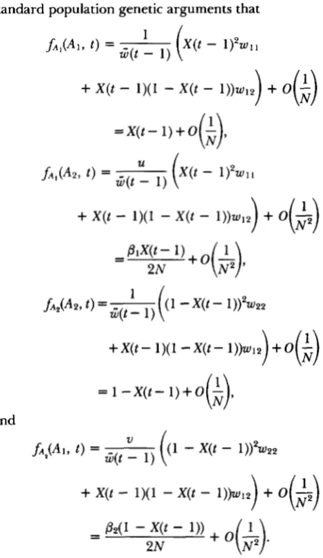
standard population genetic arguments that

+

X(t

-

1)(1

-

X ( t

-

l))w12)

+

o(;)

= X ( t

-

1)

+

o($,

+

X(t

-

1)(1

-

X(t

-

1))W]2

)

+

0

(22

-

+X(t

-

1)(1 -X@- 1))WlZ

1 +

0

(it-)

-

= l - X ( t - l > + O

-

,

( J

and

+

X(t

-

1)(1

-

X(t

-

1))w12

)

+

0

-

($2)

Letf(Aj, t ) denote the probability of picking a gene of allelic type A, regardless of the allelic type of the parental gene. It follows that

f(A1, t ) =fA1(A1, t ) +ji2(A1, t ) = X @ - l ) + O

(it.)

-

= 1

-

X(t

-

1)

+

o($

(4)

822 N . L. Kaplan, T. Darden and R. R. Hudson

coalescent is a two dimensional process. Suppose that n genes are chosen at random from the 0th generation and let Q(0) = (i, j ) if the sample consists of i A 1 alleles and j A2 alleles, 0 5 i, j 5 n, i + j = n. For t

<

0, Q(t) denotes the number of A I and AP ancestral genes of the sample in generation t . T h e total number of ancestral genes in generation t is denoted by

I

Q(t)

1.

By its very definition Q is a jump process. We define T1, T2,

. . .

to be the numbers of generations between

successive jumps and Z1,22,

. . .

the successive random states to which the process moves. T h e Q process can therefore be represented as

where S k = T,,

k

I 1. An example of an ancestral tree for a sample of size 4 is given in Figure 3.

It is clear from the definition of the Q process that

I

Q ( t )

I

never increases. Hence, the process eventually reaches either of the two states (0, 1) or (1, 0). T h e ancestral generation in which this first occurs is that generation which has the most recent common ancestor of the sample.

We now consider the joint distribution of the (Ti)

and the {Z,). Toward this end we study the distribution of Q(t

-

1) conditional on Q(t) and X ( t

-

1). There are two cases to consider:

Case 1:

I

Q(t

-

1)

I

=

I

Q ( t ) l . T h e only way that Q(t

-

1) # Q(t) is if the allelic type of at least one of the sampled genes is different (as a result of a selective mutation) than the allelic type of its parental gene. T h e probability that a sampled AP allele from generation t has an A I parental gene equals

Since j A2 genes are sampled from generation t ,

P(Q(t

-

1) = (i

+

1 , j

-

1)

I

Q ( t ) =

( i , j ) ,

X ( t

-

1))

Similarly,

P(Q(t

-

1) = (i

-

1 , j

+

1)

I

Q(t) = (Z,j), X ( t

-

1))

(7)

1

-

X ( t

-

1) p 2

\ I

=i( X ( t - 1 ) ) Z + O ( $ ) .

Furthermore, since all the other possible cases where Q(t

-

1) # Q ( t ) and 1Q(t

-

1)1 = IQ(t)I involve at least two selective mutations, these events have probabili- ties of order 1/N2.

Past

.. . . .

A , SllOIOS A alleles

FIGURE 3.-A realization of the coalescent process for a sample of size 4. The Q process changes value at the S, = %I T , ancestral generations, 1 5 j 5 5. At the Slth ancestral generation, an ancestral A? allele mutated to an A I allele, ie., the Q process moved from (2, 2) to ( 1 , 3) at the Snth and Ssth ancestral generations, common ancestors of two ancestral AS alleles occurred and so the Q process moved to ( 1 , 2) and then to ( 1 , 1 ) . At the S4th ancestral generation, an ancestral A1 allele mutated to an A2 allele and so the Q process moved to (2, 0). Finally at the Ssth ancestral generation, the most recent common ancestor of the sample occurred and the Q process moved to the state ( 1 , 0).

Case 2:

I

Q(t

-

1)

I

#

I

Q(t)

I.

In this case some of the sampled genes have common parental genes. The fraction of the genes of generation t contributed by a particular A I parental gene equals

X ( t

-

1)Wll

+

(1

-

X ( t

-

1))W12

2 N q t

-

1) +

o($)

The probability that two sampled A I genes from generation t have the same A I parental gene therefore equals

1

-

2 N X ( t

-

1) + 0

($).

Since i A1 genes are sampled from generation t ,

=(a)

1

+

₀

($).

2 2 N X ( t - 1)

(5)

Coalescent Process 823

Also, since the chance of having more than one coalescent in any generation is of order 1/N2,

P(IQ(t

-

1>1

<

IQ(t>I

-

1

I lQ(t)Ij

X(t

-

1)) = 0

($).

It follows from (6)-( 10) that the conditional distribution of Q(t

-

1) up to order 1/N is

P(Q(t

-

1) = Q(t)

I

Q(t) = (i, j ) ,

X(t

-

1))

where

( 3

i:)

h&) = -

+

-

+

- j P I X + iP2(1

-

x)

x 1 - x I - x X

(If i is less than 2, then is interpreted as 0.)

Furthermore,

P(Q(t

-

1) = (i

-

1 , j )

I

Q(t

-

1) # Q(t) = ( i , j ) , X ( t

-

1))

= q i - l j ( X ( t - 1)) + O

P(Q(t

-

1) =

( i , j

-

1)

I

Q(t

-

1) # Q(t) = ( i , j ) , X ( t

-

1))

= q ; , , - l ( X ( t - 1))

+

0 P(Q(t- l ) = ( i + 1 , j - 1)l

Q(t

-

1) # Q(t) =

( i , j ) ,

X ( t

-

1))

-

qt+l,j-1(X(t

-

1))

+

0

and

P(Q(t- l ) = ( i - l , j + 1)l

Q(t

-

1) # Q(t) = ( i , j ) ,

X(t

-

1))

-qi-l,J+l(X(t-

-

1 ) ) + 0

where

and

Thus, for large N it can be assumed as a consequence of (12) that when the Q process does jump, there are only four possible states it can jump to:

( i - l , j ) , ( i , j - l ) , ( i + 1 , j - l ) a n d ( i - l , j + 1). T h e first two states represent coalescent events and the latter two mutation events.

T h e formula for the joint distribution of the

(Ti)

and (Zi) follows from (1 1) and (12). If one conditions on the X process and uses (1 1) and (1 2) repeatedly, then

P(Ti = ti,

Zi

= ~ i , 1 I i I

k

I

Q(0) = ~ 0 )

r k

where each ti

>

0, si =

z;,=l

t,, SO = 0, each z; can take on one of four possible values which depend on the value of zi-1 and whenever s,-1

+

1 is greater than

s,

-

1, the product in (1 3) is set equal to 1. It should be noted that Ti and Zi are not independent and that the expectation in (1 3) is with respect to the distribution of the ancestral frequency process ( X ( t ) , t I 0).

We next consider the asymptotic behavior of the expectation in (1 3). As is customarily done, time is rescaled so that it is measured in units of 2N generations. It is a straightforward exercise to show that for -

N large

Hence, it follows from (13) and (14) that

/ -

ti

+

-), 1

21

= zj, 1 I i I

K

I

Q(0) = zo

2N

(6)

824 N . L. Kaplan, T. Darden and R. R. Hudson

ancestral frequency process, behaves like a two-dimensional time inhomogeneous Markov jump process.

In many cases of interest the Y process is a diffusion. For example, if the stationary frequency process ( X ( ~ N T ) , T

>

01 converges to a reversible diffusion, then { X ( - ~ N T ) , 7

>

01 also converges to a diffusion. Two examples of selective models that lead to limiting diffusions are:

Example 1 (Deleterious selection)

w11 = 1

+

s w12 = 1

+

sh w22 = 1, and

Example 2 (Overdominant selection)

w11 = 1

-

SI w12 = 1 w 2 g = 1

-

sg,

where s, s1 and sp are of order 1/2N and 0 5 h 5 1. If the limiting process is a diffusion, then it is possible to study properties of the Q process numerically. In the next section a method is described for doing such calculations and some numerical calculations are presented. A special case where this difficult numerical analysis is not necessary is also discussed.

CALCULATIONS

In this section we study the distribution of T(i, j ) ,

the sum of the lengths (measured in units of 2N

generations) of all the branches of the ancestral tree, assuming that the sample consisted of i A I alleles and

j A2 alleles (i

+

j 2 2). We first consider selective models where mutation and selection act in such a way that at equilibrium the frequencies of the two alleles remain essentially constant for long periods of time. In these cases it can be assumed that there is a constant xO(0

<

x0

<

1) such that X ( t ) = x0 for all t. These tightly regulated models are of interest because the moments of T(i, j ) are easier to compute and they may be good approximations to the moments of T(i, j ) for selective models where the frequencies of the two alleles are not tightly regulated.

If it is assumed that X ( t ) = x. for all t , then it follows from (1 5) that the limiting Q process is a time homogeneous Markov process with the following parameters. For any state ( i , j ) , the holding time in that state, TV, has a negative exponential distribution with parameter hV(x0) and the probability that the process moves from (i, j ) to (i‘, j ’ ) equals q;,j,(xo) where (i’, j ’ )

can equal (i

-

1, j ) , (i, j - 1), (i - 1, j

+

1 ) or (i

+

1,

j

-

1). It is important to note that in the tightly regulated case, the form of selection affects the limiting Q process only to the extent that it affects the value of XO. Hence, the distribution of the limiting Q process will be the same for any tightly regulated selection model having the same value of x0 and the same mutation parameters.

For some selection models, e.g., Example 1, x0 depends on and

&

For Example l , x0 satisfies the equation

~ - r ~ o ( l

-

XO)(XO

+

h ( l

-

2x0))

(16)

-

P I X 0

+

P2(1

-

xo) = 0,

where a = 2Ns (EWENS 1979). If x0 is close to one, then it is well known (EWENS 1979) that

x()= 1

- _ _ _

~ ( l

-

h)’

U

while if s

>

0 and h = 1. then r

For other selection models x0 may not depend on the mutation parameters. This is true for Example 2 if u

and v are small when compared to s1 and s2, since in this case

x0 =

-.

SP

SI

+

SP

T h e conditions under which the approximating diffusions in Examples 1 and

2

behave as if they converge to a deterministic equilibrium point have been discussed by many authors (NORMAN 1975; KURTZ 198 1) and the interested reader should consult their papers for details. Loosely speaking, the diffusion will behave in this way if the infinitesimal mean is large compared to the infinitesimal variance.

T h e following representation for

T(i,

j ) is a direct consequence of the Markov property of the limiting Q process. If we consider what happens when the process first changes value, then

T(i,

j ) = (i

+

j)Tq

+

T(Z,.),

where Tq is the holding time in state (2, j ) , Z, is the random state to which the process moves and if 2 , =

(i’, j ’ ) , then T ( Z y ) is an independent random variable having the same distribution as T(i’, j ’ ) .

Recursions for the mean and variance of T(i, j ) are easy to obtain from (1

7).

Let Mq denote the mean of T ( i , j ) and Vq its variance. Then

and

(7)

Coalescent Process 825

Equations 18 and 19 are not useful for studying the behavior of

MI^.

and V , if n is large. It is easier to study the evolution of the (2 process directly. It is not hard to show that the behavior of the mean and variance of T ( i , j ) for large samples is the same as in the neutral case. That is, the mean of T(i,

j )

grows like log(i

+

j )

and its variance remains bounded.

For small samples, it is necessary to solve the recursions in (1 8) and (1 9) for particular parameter values. Since it may commonly be the case that one cannot distinguish between the two alleles, we assume that the number of A1 alleles in the sample is random with a binomial distribution. T h e quantities tabulated in Table 1 are therefore

Mn(xo) =

i

(1)

xh(1

-

xo)n-iMin-i,

i=o i C /

and

T h e results in Table 1 show that the values of M,(xo)

and Vn(xo) only differ significantly from their values in the neutral case when both /31 and /32 are small.

Furthermore, the closer x0 is to 0 or 1, the smaller

PI

and /32 have to be in order for M,(xo) and Vn(x0) to differ from their neutral values.

It is easy to explain why small values of /31 and /32

lead to ancestral trees which do not look neutral. If selective mutations are rare, then most of the state changes in the Q process result from common ancestor events. Hence, with high probability all the A I alleles and all the AQ alleles will coalesce, resulting in just two ancestral genes; one of each allelic type. In order for these two ancestral genes to have a common ancestor, it is necessary for a selective mutation to occur first. If /31 and /32 are small, then this event takes a long

time to occur and so the ancestral tree will not look neutral.

In those cases where x0 depends on P I and ,f32 the

above behavior may not hold. T o see what can happen we consider Example 1 of the previous section. For a sample of size 2 the equations for MZ0, M l l and MO2

are easy to solve. Indeed,

M20 = 2x0 2P41 -

X 0 ) M I 1

1

+

2P2( 1

-

xo)

+

1

+

2p2( 1

-

xo)’

and

P2(

1

-

x0)3

1

+

2PlXO

+

1

+

2/34 1

-

xo)

TABLE 1

Mean (M,,(xo)) and variance ( V . ( ~ O ) ) of the total time in the genealogy of a random sample of n genes, assuming tight

regulation

n = 2 n = 20

- 81 81 x 0 M z ( X 0 ) V * ( X O ) Mno(x0) Vzo(x0)

100.0 100.0 0.5 2.0 4.0 7.1 6.4

0.1 1.8 3.4 6.5 5.4

0.05 1.9 3.6 6.5 5.4

10.0 10.0 0.5 2.1 4.2 7.3 6.7

0.1 1.8 3.4 6.6 5.4

0.05 1.9 3.6 6.8 5.8

1.0 1.0 0.5 2.5 6.8 8.4 9.9

0.1 1.9 3.4 6.8 5.5

0.05 1.9 3.7 6.8 5.8

0.1 0.1 0.5 7.0 99.0 17.5 127.0

0.1 2.2 5.2 8.5 10.5

0.05 2.0 3.9 7.5 6.8

0.01 0.01 0.5 52.0 7704.0 108.0 10208.0

0.1 5.8 163.0 26.0 483.0

0.05 2.9 24.0 13.5 102.0

1.0 100.0 0.5 1.0 1

.o

3.8 1.7

0.1 1.8 3.2 6.4 5.2

0.05 1.9 3.6 6.7 5.8

100.0 1.0 0.1 0.85 0.60 3.6 1.2

0.05 1.6 2.4 5.8 4.0

80.0 5.0 0.5 1.1 1.3 4.2 2.0

0.1 2.0 3.8 6.9 6.1

For comparison the mean and variance of the time in the genealogical history of sample from a selectively neutral model is 2.0 and 4.0, for a sample of size 2, and 7.1 and 6.4, for a sample of size 20.

Suppose that / 3 1 and

0 2

are both small and that x0

satisfies (16a). In this case, a must be large in order for the frequency of the A I to be tightly regulated. It is not difficult to show under these conditions that

X I 3 4 2 0

=

2, xo(1

-

X 0 ) M I l

=

0

and (1

-

~ o ) ~ M ~ ~

=

0.

Thus, MZ(x0)

=

2 regardless of how small

p1

and

p2

are.

Knowing the allelic composition of the sample also affects the conclusions about the sample’s genealogy. For example, suppose that both members in a sample of size 2 are the same allelic type. Suppose also that

PI

=

PZ

=

/3

=

0, and x0

=

1. Then it is not difficult to show that

M2o

=

2

and

l M o 2

=

2(1

-

~ 0 )

+

4(1

-

XO

+

p).

Thus, if one picked two genes of the common allelic type, then the ancestral tree looks neutral. If, on the other hand, one picked two genes of the rare allelic type, then the ancestral tree looks much smaller than a neutral tree.

(8)

826 N. L. Kaplan, T. Darden and R. R. Hudson

pose at locus A there are two classes of alleles which are denoted A1 and Az. Class A I consists of alleles A l l , AI,,

. . .

and class A2 consists of alleles A21, A22,

. . . .

Suppose that every selective mutation of an A I allele gives rise to a new allele of the A2 class and vice versa. In addition each neutral mutation gives rise to a new allele within the same class. HARTL and CAMPBELL (1 982) showed under these assumptions that the distribution of the number and frequencies of AI alleles in a random sample from the AI class follows an infinite alleles distribution (EWENS 1972) where

A similar result holds for a sample from the A2 class with

HARTL and CAMPBELL proved this result without using the coalescent process. Their arguments however, provide no information about the distribution of the number of segregating neutral sites in the sample. For the model considered by HARTL and CAMPBELL, our analysis shows that the expected number of neutral segregating sites in a sample of n genes from the AI class equals 2NpE(T(n, 0)).

We now examine selective models where the limiting Y process is a diffusion which is not tightly regulated. In these cases one can show that for any n 2 2, the functions, ( F q ( t , x) = P(T(i, j )

>

t l Y ( 0 ) = x), 2 I i

+

j 5 n ) are the solution of the following system of partial differential equations

F,(t, x)

+

- b@) ₂

a2

_F,(t,_x)

2 ax

where t

>

0 , O

<

x

<

1 and 2 5 i + j 5 n.

T h e derivation of (20) relies on the same kinds of Taylor series arguments that are used to study the distribution of a hitting time for a diffusion process

(KARLIN and TAYLOR 1981).

There are several difficulties in solving (20) numer-

ically. First, the coefficient of the second order term equals zero at the boundaries, i e . , b(0) = b(1) = 0. Second, the boundary conditions, ( F , ( t , 0) and FG(t, l ) , t

>

01 are unknown. Finally, the right-hand side of (20) explodes as x approaches 0 and 1. For these reasons standard software packages for solving partial differential equations cannot be used and so alternative methods need to be developed.

Since none of the coefficients in (20) are time de- pendent, it is not difficult to obtain from (20) a system of equations for each moment of T ( i , j ) . For example, if M , ( x ) = E ( T ( i , j )

I

Y ( 0 ) = x), then integrating both sides of (20) with respect to t leads to

where 0

<

x

<

1 and 2 5 i

+

j 5 n. To obtain equations for the higher moments of T(i, j) one multiplies both sides of (20) by an appropriate power of t before integrating.

For the same reasons given above, standard software packages for solving systems of equations such as those in (21) cannot be used. In a forthcoming paper (DARDEN, KAPLAN and HUDSON 1988), a numerical method for solving (21) is described. This method is patterned after the LU decomposition for tridiagonal matrices (PRESS et al. 1988).

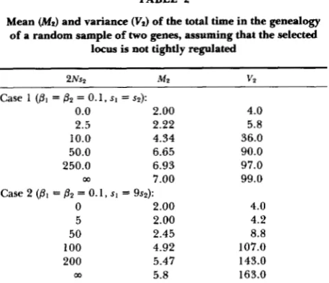
To illustrate the numerical results the following examples are considered. In Table 2 the analogs of M2(xO) and VZ(x0) are calculated for a sample of size 2, assuming the selection model of example 2. These quantities are

M z =

(;)

i'

M i 2 - z ( ~ ) ~ i ( l

-

x)'"p(x)dx

;=0

and

v,

=

;

(;)

J 1 L;2-i(x)x1(1

-

x ) Z - y ( x ) d x

-

( M , ) * ,

i=O

where Lq(x) = E (T(i, j)'I Y(0) = x ) and p ( x ) is the stationary density of the diffusion.

Two cases were considered. In the first case P I = P 2 = 0.1 and s1 = sg, while in the second case P I = P 2 =

(9)

Coalescent Process 827

TABLE 2 10 1

Mean (MI) and variance (Vr) of the total time in the genealogy

of a random sample of two genes, assuming that the selected locus is not tightly regulated

2 N ~ 2 MP V2

Case 1 (PI = B2 = 0.1, sI = s~):

0.0 2.00 4.0

2.5 2.22 5.8

10.0 4.34 36.0

50.0 6.65 90.0

250.0 6.93 97.0

m 7.00 99.0

Case 2 (Dl = p2 = 0.1, S, = 9 ~ ~ ) :

0 2.00 4.0

5 2.00 4.2

50 2.45 8.8

100 4.92 107.0

200 5.47 143.0

m 5.8 163.0

For both of these cases the limiting diffusion is associated with

the overdominant selection model of Example 2.

0.5, whereas for the second case it equals 0.1. T h e results in Table 2 show that the values of M ~ ( X O ) and

V2(x0) are good approximations to M2 and V2 so long

as 2Ns2

>

50 in case 1 and 2Ns2

>

200 in case

2.

T o provide a visual impression of the tightness of the regulation of the frequency process, the density of the stationary distribution of the limiting diffusion for case 1 is plotted in Figure 4 for four values of 2Ns2.

It is evident that there is some variability when 2Ns2

equals 50, and yet the tight-regulation approximation is quite accurate.

Up until now we have considered selection models where the infinitesimal variance of the approximating diffusion is not large. For some models however, this may not be true. For example, the random environ- ment models studied by GILLESPIE (1978) lead to diffusions whose infinitesimal means and variances are of the form

a ( x ) = x ( l - x ) C

c

A + B

G

- " X

)I

and

b ( x ) = CX2(1

-

x)2, where A , B and C are constants.

Diffusions of this type can be thought of running on a different time scale and so it is appropriate to rescale time. Thus, suppose that the ancestral frequency process {X(-2N7), 7

>

O ] converges weakly to

a process {Y(C7), 7

>

01, where Y is a diffusion and C is a constant. If C is sufficiently large, i.e., the diffusion is running on a faster time scale, then it follows from (1 4) and (1 5) that the coalescent process can again be approximated by a time homogeneous Markov process. The joint density of the holding time in any state

0.0 0.2 0.4 0.6 0.8 I .o

Frequency

FIGURE 4.-The stationary density of the limiting diffusion associated with the overdominant selection model of Example 2.

and the random state to which the process jumps is

= e --t

1'

hz(u)P(u)du

(s'

h z ( U ) q z l ( U ) p ( U ) d U

where p ( u ) is the stationary density of the approximating diffusion, Y.

DISCUSSION

Restriction mapping and DNA sequencing of samples of genes from populations give information that is more detailed and less ambiguous than the information from allozyme studies. These new molecular techniques also provide information about the age and genealogical relationships of alleles (e.g., SHAW

and LANGLEY 1979; STEPHENS and NEI 1985;

AQUADRO et al. 1986). Effective use of this new type of information requires an understanding of the genealogical relationships expected under competing population genetic hypotheses that might explain the observed molecular genetic variation. Under some simple genetic models without selection, many statistical properties of the process describing the genealogical history of samples are known (WATTERSON

1975; KINCMAN 1982a, b; TAVARI? 1984). T h e pur- pose of this investigation is to study properties of this process for population genetic models which are not selectively neutral.

T h e distribution of the coalescent process for models with selection depends on the distribution of the frequencies of alleles in the ancestral generations. For many two-allele selective models, e.g., examples 1

(10)

828 N. L. Kaplan, T. Darden and R. R. Hudson

Some simplification is possible if it can be assumed that the allelic frequencies do not vary from generation to generation, ie., they are tightly regulated. For selection models of this type, the coalescent process is a time homogeneous Markov jump process whose distribution only depends on the mutation rates and the equilibrium frequency, regardless of the form of selection. In this case the mean and variance of T each satisfy a system of linear equations which is much easier to solve. Furthermore, the results in Tables 1 and 2 suggest that the values obtained assuming tight regulation are good approximations even when the allelic frequencies are not that tightly regulated.

T h e arguments for the tightly regulated case can be easily generalized to k-allele models, k

>

2 . If the allelic frequencies are not tightly regulated then the results do not generalize since the limiting ancestral frequency process, ( Y ( t ) , t

>

0), is not generally known to be a diffusion for

k

>

2 .

If, for the tightly regulated case, the allelic frequencies do not depend on the mutation parameters,

01(=2Nu) and &4=2Nv), for example under models of strong balancing selection, then the mean and variance of T differ substantially from their values in the neutral case only when the mutation parameters,

p1

and &, are small. If, on the other hand, the allelic frequencies depend on the mutation parameters, then the mean and the variance of T may not differ significantly from their neutral values regardless of how small 01 and 0 2 are. The mutation-selection balance model illustrates this behavior.

For neutral models, an unbiased estimate of 2 N p is

S/(2C';-' I/j), where S is the number of segregating sites in a random sample of n genes and 2 I/' is the expected value of T for a neutral model for a random sample of n genes. If in fact some of the genetic variation is not selectively neutral, then an unbiased estimate of 2 N p is S,,,/E(T), where S,,, is the number of segregating selectively neutral sites and

E ( T ) is the expected value of T for the selective model. Thus, under the selective model, the neutral estimate is biased in the following two ways. First, the observed value of S is too large since it is the sum of the numbers of segregating neutral sites (S,,,,) and segregating selective sites (&,I), If the number of segregating selec-

tive sites is small compared to the number of segregating neutral sites, e.g. if

P1

and 0 2 are small com-

pared to 2 N p , then using the observed value of S instead of S,,,, will not introduce much error. Sec- ondly, under a selective model, the expected value of T may, in fact, be much larger than 2 l/j, and so the neutral estimate of 2 N p may be too large. If 01

and

Pz,

are very small, then this bias could be substan- tial (Table 1).

The models studied in this paper assume that all sites are completely linked. Clearly, it is important to

introduce recombination into the analysis and in particular to determine the behavior of the coalescent process for neutral sites not completely linked to a site at which selection is operating. In a companion study in this journal this problem is addressed (HUDSON and KAPLAN 1988).

L I T E R A T U R E CITED

AQUADRO, C. F., S. F. DEESE, M. M. BLAND, C. H. LANGLEY and C. C. LAURIE-AHLBERG, 1986 Molecular population genetics of the alcohol dehydrogenase gene region of Drosophila mela-

nogaster. Genetics 1 1 4 1 165-1 190.

BILLINGSLEY, P., 1968 Convergence of Probability Measures. Wiley, New York.

CHAKRAVARTI, A,, S. C. ELBEIN and M. A. PERMUTT, 1986

Evidence for increased recombination near the human insulin gene: Implication for disease association studies. Proc. Natl.

Acad. Sci. USA 83: 1045-1049.

DARDEN, T., M. L. KAPLAN and R. R. HUDSON, 1988 A numerical method for calculating moments of coalescent times in finite populations with w selection. J Math Biol (in press).

EWENS, W . J., 1972 The sampling theory of selectively neutral alleles. Theor. Popul. Biol. 3: 87-1 12.

EWENS, W. J., 1979 Mathematical Population Genetics. Springer-

Verlag, New York.

GILLESPIE, J. H., 1978 A general model to account for enzyme variation in natural populations. V. T h e SAS-CFF model. Theor. Popul. Biol. 14: 1-45.

GILLESPIE, J . H., 1986 Variability of evolutionary rates of DNA.

Genetics 113: 1077-1091.

HARTL, H. L., and R. B. CAMPBELL, 1982 Allele multiplicity in

simple Mendelian disorders. Am. J. Hum. Genet. 34: 866-873.

HUDSON, R. R., 1987 Estimating the recombination parameter of

a finite population model without selection. Genet. Res. 5 0 245-250.

HUDSON, R. R., and N. L. KAPLAN, 1986 On the divergence of

alleles in nested subsamples from finite populations. Genetics 113: 1057-1076.

HUDSON, R. R., and N. L. KAPLAN, 1988 The coalescent process

in models with selection and recombination. Genetics 120:

819-829.

HUDSON, R. R., M. KREITMAN and M. A G U A D ~ , 1987 A test of neutral nrolecular evolution based on nucleotide data. Genetics 116: 153-159.

KAPLAN, N. L., and R. R. HUDSON, 1987 On the divergence of

genes in multigene families. Theor. Popul. Biol. 31: 178-194. KARLIN, S . , and H. M . TAYLOR, 1981 A Second Course in Stochastic

Processes. Academic Press, New York.

KIMURA, M., 1969 The number of heterozygous nucleotide sites

maintained in a finite population due to a steady flux of

mutations. Genetics 61: 893.

KINGMAN, J. F . C., 1982a On the genealogy of large populations. J. Appl. Prob. A19: 27-43.

KINGMAN, J. F. C . , 1982b The coalescent. Stochastic Process. Appl. 13: 235-248.

KREITMAN, M., 1983 Nucleotide polymorphism at the alcohol

dehydrogenase locus of Drosophila melanogaster. Nature 304:

412-417.

KURTZ, T. G., 198 1 Approximation of Population Processes. Society for Industrial and Applied Mathematics, Philadelphia.

NORMAN, F . , 1975 Approximation of stochastic processes by

Gaussian diffusions and applications to Wright-Fisher genetic

models. SIAM J. Appl. Math. 2 9 225-242.

(11)

Coalescent Process 829

VETTERLING, 1988 Numerical Recipes in C: The Art of Scient@ TAVARP, S., 1984 Line-of-descent and genealogical processes, and

Computing. Cambridge University Press. their applications in population genetic models. Theor. Popul.

variation in restriction maps of Drosophila mitochondrial WATTERSON, G . A., 1975 On the number of segregating sites in

DNAs. Nature 281: 695-699. genetical models without recombination. Theor. Popul. Biol.

SHAW, D. M., and C. H. LANGLEY, 1979 Inter- and intraspecific Biol. 2 6 119-164.

STEPHENS, J. C., and M. NEI. 1985 Phylogenetic analysis of poly- 10: 256-276.

morphic DNA sequences at the Adh locus in Drosophila mela-