ABSTRACT
HUANG, YUFAN. Spreading Processes in Complex Networks: Speed, Competition, and Privacy. (Under the direction of Dr. Huaiyu Dai).
Spreading processes exist in many real-world systems. It has been recognized by many researchers as an important topic in their fields. However, theoretical understandings of spreading processes in recent emerging complex systems modeled by complex networks are essentially lacking. In this dissertation, we explore and study the properties of spread-ing processes in some burgeonspread-ing complex network systems.
The first part of this dissertation is dedicated to information spreading in multi-plex networks. Multimulti-plex networks, a special type of multilayer networks, possess several unique features like multi-channel communication and information synchronization that can affect the way information spreads among nodes in the network. In Chapter 2, con-sidering the gossip mechanism, the information spreading speed in multiplex networks is analyzed for synchronous and asynchronous time models. In the synchronous time model, the informed probability model is proposed to help understand the spreading behavior in multiplex networks. A new metric, named multiplex conductance, is defined and used to measure the time required for a piece of information to be received by all nodes. A novel multiplex network design that dramatically facilitates the information spreading process is discovered through rewiring of interlayer connections. The trade-off between the additional layer cost and the spreading efficiency improvement is investigated from both the user’s and network designer’s perspectives. In the asynchronous time model, a qualitative comparison study is performed in terms of the average information spreading time. The number of layers, the average degree of each layer, and the similarity between layers are found to influence the speed of information flows across the multiplex network. Simulations on both synthetic and real networks conform to our findings.
spreading process is influenced by the structural similarity between the two layers in this case. A higher similarity indicates a stronger immune response so that viral infections are harder to sustain. When both layers are spatial random networks, the immune response is able to stop viruses in a more effective manner by blocking the spreading paths of viruses. The competition between these two processes is then generalized to a multi-tissue environment which is modeled by a multi-cluster network. By considering each cluster in the network as a super node, theoretical approximations can be obtained. Two types of cluster distributions are considered including homogeneous and heterogeneous clusters. A double phase transition is observed in terms of the final outcome when there exists a giant cluster in the network. All theoretical approximations and discoveries are verified through extensive simulations.
In the last part, privacy is explored in the context of information spreading. Gossip protocols, a randomized information distribution algorithm, are often believed to be effective in protecting the identify of the information source. However, no theoretical justification has been provided to support this argument. In Chapter 4, the differential privacy framework is adopted to investigate how well gossip protocols protect the privacy of information source. Lower bounds of the differential privacy of gossip protocols in general networks are derived for both the synchronous and asynchronous time settings. Our results suggest that more information about the information source can be leaked to the adversary in networks with a large diameter in the asynchronous setting. Such networks are more prone to the source identification attack when the whole spreading process is monitored. The differential privacy of gossip protocols in wireless networks with unreliable communications is also explored, and it is found that artificial interference can protect the privacy of the source identity at the cost of slowing the spreading process. In the end, the delayed monitoring model is considered for the attacker, and theoretical results imply that a longer delay leads to a stronger differential privacy guarantee by the gossip protocols in protecting the source identity.
Spreading Processes in Complex Networks: Speed, Competition, and Privacy
by Yufan Huang
A dissertation submitted to the Graduate Faculty of North Carolina State University
in partial fulfillment of the requirements for the Degree of
Doctor of Philosophy
Electrical Engineering
Raleigh, North Carolina 2019
APPROVED BY:
Dr. Brian Hughes Dr. Dror Baron
Dr. Ruian Ke Dr. Wenye Wang
Dr. Huaiyu Dai
DEDICATION
BIOGRAPHY
ACKNOWLEDGEMENTS
First, I would like to show my deepest gratitude and appreciation to my advisor, Professor Huaiyu Dai, for his patient guidance and continuous support over my PhD study. His encouragement has guided me through the ups and downs of my research. Without him, I would not have come this far and finished this dissertation. He also provides a role model of integrity and humility that I believe I will continuously learn and pursue the rest of my life. It is my great honor and fortune to have worked with him for seven years. I also want to express my sincere thankfulness to Professor Ruian Ke. In my last half of PhD journey, when I started a new cross-disciplinary research project that I have never touched, he provided detailed instructions and great suggestions to direct me. More importantly, I also learned how to collaborate with others in a positive and optimistic manner from him.
My heartfelt appreciation also goes to Professor Dror Baron, Professor Brian Hughes, and Professor Wenye Wang for their insightful advice and feedback. I want to also thank all the faculty and staff members in the department of Electrical and Computer Engi-neering of NC State University for all the amazing courses and the excellent study and research environment.
Furthermore, I am lucky to have encountered so many great friends and colleagues at NC State: Xiaofan He, Juan Liu, Huazi Zhang, Richeng Jin, Qi Jia, Hong Xiong, Ali Rahmati, Seyyedali Hosseinalipour, Srinjoy Chattopadhyay, and Anuj Nayak. Not only have we had many great discussions about research, we shared countless happy moments together. My journey here would not be so delightful without their friendships.
Special thanks to the financial support from Army Research Office (under Grant W911NF-17-1-0087) and US National Science Foundation (under Grants ECCS-1307949, EARS-1444009, and CNS-1824518).
TABLE OF CONTENTS
LIST OF TABLES . . . vii
LIST OF FIGURES . . . viii
Chapter 1 Introduction . . . 1
1.1 Information Spreading in Multiplex Networks . . . 1
1.2 Competition Between Virus Infection and Immune Protection Processes . 3 1.3 Privacy in Information Spreading . . . 4
1.4 Organizations . . . 5
Chapter 2 Gossip-based Information Spreading in Multiplex Networks 6 2.1 Problem Formulation . . . 7
2.1.1 Basic Models . . . 7
2.2 Synchronous Gossip in Multiplex Networks . . . 10
2.2.1 Informed Probability Model . . . 10
2.2.2 Idealized Information Spreading Time . . . 14
2.2.3 Multiplex Conductance Evaluation and Performance Improvement 21 2.2.4 Layer Cost and Information Spreading Efficiency . . . 26
2.3 Asynchronous Gossip in Multiplex Networks . . . 34
2.3.1 Qualitative Spreading Time Comparison . . . 34
2.3.2 Layer Similarity and Network Diameter . . . 42
2.3.3 Connectivity of Multiplex Networks . . . 43
2.3.4 Simulation Results . . . 45
2.4 Conclusions . . . 50
Chapter 3 Network Analysis of Virus-innate Immune Interaction Process 53 3.1 Problem Formulation . . . 53
3.1.1 Network Models . . . 54
3.1.2 Virus-innate Immune Interaction Process . . . 56
3.2 Virus-innate Immune Interaction in a Single Network . . . 58
3.2.1 ER Layers . . . 58
3.2.2 GR Layers . . . 65
3.3 Competition in a Multi-cluster Network . . . 65
3.3.1 Homogeneous Multi-Cluster Networks . . . 66
3.3.2 Heterogeneous Multi-cluster Networks . . . 67
3.4 Numerical Simulations . . . 68
3.4.1 Single Network with ER Layers . . . 68
3.4.2 Single Network with GR Layers . . . 69
3.5 Conclusion . . . 75
Chapter 4 Quantifying Differential Privacy of Gossip Protocols in Gen-eral Networks . . . 78
4.1 System Model Overview . . . 79
4.1.1 Time Model . . . 79
4.1.2 Observation Model . . . 80
4.1.3 Privacy Model . . . 80
4.1.4 Prediction Uncertainty . . . 82
4.2 Main Results . . . 82
4.2.1 Differential Privacy of Gossip Protocols in General Networks . . . 83
4.2.2 Differential Privacy of Private Gossip Protocol . . . 85
4.2.3 Differential Privacy of Standard Gossip Protocol . . . 88
4.2.4 Differential Privacy of Gossip Protocols in Wireless Networks . . . 90
4.2.5 Differential Privacy of Gossip Protocols in Delayed Monitoring . . 93
4.3 Conclusion . . . 96
Chapter 5 Summary and Future Work . . . 97
5.1 Conclusions . . . 97
5.2 Future Works . . . 98
References . . . 100
Appendix . . . 108
Appendix A Appendix for Chapter 2 . . . 109
A.1 Proof for Lemma 1 . . . 109
A.2 Proof for Corollary 1 . . . 113
LIST OF TABLES
Table 2.1 Important Notations with Definitions . . . 34
Table 2.2 Statistics for Multiplex Network 1 . . . 50
Table 2.3 Statistics for Multiplex Network 2 . . . 51
Table 2.4 Average Spreading Times for Multiplex Network 1 . . . 51
LIST OF FIGURES
Figure 2.1 Gossip Algorithm in a Two-layer Multiplex Network . . . 9
Figure 2.2 From Multiplex Network to Aggregated Multigraph . . . 15
Figure 2.3 Proposed Ring-Ring Structure r= 4 . . . 22
Figure 2.4 Efficiency Improvement for Proposed Ring-Ring . . . 23
Figure 2.5 Ring-Complete and Ring-PA . . . 25
Figure 2.6 Information Spreading in Multiplex Networks with Identical Ring Graphs 27 Figure 2.7 User Aspect . . . 29
Figure 2.8 Enlargement of Fig. 2.7 . . . 30
Figure 2.9 Designer Aspect . . . 32
Figure 2.10 Enlargement of Fig. 2.9 . . . 33
Figure 2.11 Impact of Layer Number: Multiplex SF networks (r = 2) . . . 44
Figure 2.12 Impact of Layer Number: Multiplex ER networks (p= 1.1 logn n) . . . . 44
Figure 2.13 Impact of Layer Similarity: Multiplex SF Networks (r= 2) . . . 45
Figure 2.14 Impact of Layer Similarity: Multiplex SF networks (r = 5) . . . 46
Figure 2.15 Impact of Layer Similarity: Multiplex SF networks (r = 10) . . . 46
Figure 2.16 Impact of Layer Similarity: Multiplex ER networks (p= 1.1 logn n) . . . 47
Figure 2.17 Impact of Layer Similarity: Multiplex ER networks (p= 2 lognn) . . . . 47
Figure 2.18 Impact of Average Node Degree: Multiplex SF networks . . . 48
Figure 2.19 Impact of Average Node Degree: Multiplex ER Networks . . . 48
Figure 2.20 Impact of Adding Layers: 5-layer Case . . . 48
Figure 2.21 Impact of Average Node Degree: 5-layer Case . . . 48
Figure 3.1 A Multi-cluster Network Example . . . 55
Figure 3.2 The Multiplex Network Framework for the Dynamics of Virus Infection and the IFN Response . . . 57
Figure 3.3 βc v.s. γ and Sim (¯kI = 5,¯kP = 4) . . . 62
Figure 3.4 From a Homogeneous cluster Network to a Heterogeneous Multi-cluster Network . . . 68
Figure 3.5 Ratio of Recovered Nodes R(∞) . . . 69
Figure 3.6 Ratio of Protected Nodes P(∞) . . . 69
Figure 3.7 The Effectiveness of the IFN Response Under Different Assumptions and Topologies of the Network . . . 70
Figure 3.8 The IFN response effectively halt/suppresses virus spread in networks with two GR graphs when RF > RI . . . 71
Figure 3.9 Visualization of Simulations of the Multiplex Networks . . . 72
Figure 3.12 Star Multi-cluster Network with ER Clusters . . . 74
Figure 3.13 Star Multi-cluster Network with GR Clusters . . . 74
Figure 3.14 Homo ER Multi-cluster Network with ER Clusters . . . 74
Figure 3.15 Homo ER Multi-Cluster Network with GR Clusters . . . 74
Figure 3.16 Hetero ER Multi-cluster Network with ER Clusters . . . 75
Figure 3.17 Hetero ER Multi-cluster Network with GR Clusters . . . 75
Figure 3.18 R(∞) for Homo ER Multi-cluster Network with Two-layer ER Clusters 76 Figure 3.19 P(∞) for Homo ER Multi-cluster Network with Two-layer ER Clusters 76 Figure 3.20 R(∞) for Hetero ER Multi-cluster Network with Two-layer ER Clusters 76 Figure 3.21 P(∞) for Hetero ER Multi-cluster Network with Two-layer ER Clusters 76 Figure 3.22 R(∞) for ER Multi-cluster Network with Two-layer GR Clusters . . 76
Figure 3.23 P(∞) for ER Multi-cluster Network with Two-layer GR Clusters . . 76
Figure 4.1 Sensor Monitoring and Observations . . . 81
Figure 4.2 Trade-off Between Differential Privacy and Spreading Speed for Stan-dard Gossip in the Synchronous Setting . . . 93
Figure 4.3 Trade-off Between Differential Privacy and Spreading Speed for Stan-dard Gossip in the Asynchronous Setting . . . 93
Figure 4.4 Trade-off Between Differential Privacy and Spreading Speed for Pri-vate Gossip in the Synchronous Setting . . . 94
Figure 4.5 Trade-off Between Differential Privacy and Spreading Speed for Pri-vate Gossip in the Asynchronous Setting . . . 94
Figure A.1 1-Separation for Layer 1 . . . 114
Figure A.2 1-Separation for Layer 2 . . . 114
Figure A.3 Balanced Separation when |DS(1)|=|DS(2)|= 1 . . . 115
Figure A.4 Balanced Separation when |DS(1)|= 2 and|D(2)S |= 1 . . . 115
Figure A.5 Balanced Separation |D(1)S |=|DS(2)|= 2 . . . 116
Chapter 1
Introduction
Spreading processes are pervasive in nature and human society and have captured the attention of researchers from different areas. Sociologists consider gossip, a typical way of exchanging information, as the critical social bond that helps formulate a large hu-man society [1]. Discovering the way information flows across people can help researchers understand how the society evolves and functions. In epidemiology, when an epidemic arises, quarantine and vaccination strategies require a mathematical model of the corre-sponding epidemic spreading process. In computer science, it is vital to design effective data distribution algorithms for tasks like distributed machine learning. Despite exist-ing results, recent technology developments in social networks, biology, and distributed algorithms call for more advanced understandings of spreading processes in these new complex systems. In this dissertation, we seek to explore spreading processes from three perspectives, speed, competition, and privacy, to provide insights for future studies in this area.
1.1
Information Spreading in Multiplex Networks
for propaganda. Recent phenomenal popularity of social networks sets a trend of using Facebook and Twitter to post opinions, through which words can be disseminated on an unprecedented scale and range. Therefore, with increasingly complicated interconnections and interactions, various kinds of communication networks and social media have formed a new network structure that enables people to spread and receive information simulta-neously through multiple channels and platforms. Recently, multilayer network models have been introduced to facilitate relevant studies on emerging inter-connected complex networks [2–5]. Extensive attention has been paid to multiplex networks, a special type of multilayer networks, for which all layers share the same set of nodes. In practice, the same set of nodes may correspond to individuals who can communicate through multiple networks or platforms, and duplicates of the same node may represent different commu-nication devices or social accounts a person may have. In the first part of this thesis, the information spreading process in multiplex networks is explored.
As a common tool for studying information spreading in the single network, the com-partmental epidemic models (e.g., infected-recovered (SIR) or susceptible-infected-susceptible (SIS) models) have been utilized to discover how the multiplex net-work structure affects the information spreading process [6–11]. For example, Cozzo et al. [9] proposed a contact-based epidemic-like information spreading model in multiplex networks. It demonstrated that the critical point for the network to have a constant por-tion of informed nodes is determined by the layer whose contacting probability matrix has the largest eigenvalue. In [7], Zhao et al. considered a spreading process on a two-layer multiplex network with a certain similarity between these two layers and showed that a positive degree-degree correlation between two layers may lead to a smaller infection size in the end.
esti-mated through a new metric called multiplex conductance. Qualitative comparisons are conducted for the asynchronous gossip in different multiplex networks. Results in both models suggest that information spreads faster in multiplex networks compared to its counterpart in a single network.
1.2
Competition Between Virus Infection and
Im-mune Protection Processes
A single spreading process is discussed in Chapter 2. However, in nature, it is very common that multiple spreading processes are coupled, either for cooperation or for competition. For example, living organisms are constantly exposed to a wide range of viral pathogens. As a result, sophisticated and highly optimized immune defense systems have been developed to protect hosts from pathogen invasions. The host innate immune response, particularly the interferon (IFN) response, represents the first line of defense against viruses [18]. Viruses infect a host by entering host cells to replicate and pack-age their genomes to form infectious viral particles. These newly produced viruses then spread to infect other susceptible cells. To defend against such an invasion, host cells pro-duce recognition molecules to bind to intracellular viral genetic materials. The binding would trigger signals to the host genome, leading to activation of numerous genes that produce proteins to form an antiviral response. Importantly, IFN molecules are produced in infected cells and secreted extracellularly. They then act as messenger molecules to activate antiviral responses in neighboring cells protecting them from viral infection [19]. The IFN signaling to protect susceptible cells is thus an analogy to the vaccination of sus-ceptible individuals at the population level. Since both viruses and the IFN molecules are generated from infected cells, the virus-IFN interaction can be viewed as a competition process in spreading among host cells.
observations [25–27]. However, a theoretical foundation to understand the mechanism by which IFN signaling stops a viral invasion and the key parameters that determine its effectiveness is lacking. Chapter 3 is devoted to investigating the IFN response to the viral invasion. A two-layer multiplex network is proposed and adopted to study the competition between viruses and IFN. Theoretical approximations about the competition process are developed along with the verification from numerical simulations. The competition is even generalized to the multi-cluster setting to discover its systematical behaviors.
1.3
Privacy in Information Spreading
Besides spreading speed and competition, private information spreading is also consid-ered in this dissertation. Recent exposure of the Facebook user data leakages accelerated people’s awareness of privacy issues and galvanized researchers. On the one hand, compa-nies need data to build models for their services. On the other hand, analyzing the data potentially reveals certain private information, which can be further inferred by an adver-sary through attacks such as the linkage attack. To address the balance between privacy and data usage, differential privacy is proposed in [28]. Differential privacy is a widely adopted framework for quantifying the privacy guarantees of privacy-preserving data analysis algorithms. Differential privacy has been extensively used in machine learning and data analysis for designing privacy-preserving algorithms. However, besides the con-ventional passive data privacy, privacy concerns also arise in active information-spreading behaviors. For example, people wish to remain anonymous in the online world when publishing sensitive information. Private information is often shared by different organi-zations during collaboration and needs to remain anonymous to outsiders. This kind of privacy concerning identity during the information distribution process is considered as information source privacy and has been recognized and investigated recently.
Information source privacy is firstly studied in [29] using the differential privacy frame-work. The information distribution model used in this work is gossip protocols, a typical family of randomized information diffusion algorithms. Though great efforts have been paid to the estimation of the information spreading time of gossip protocols [30,31], their privacy guarantee is barely touched. Current privacy results of gossip protocols [29] are derived based on the complete network assumption.
Chap-ter 4, differential privacy of gossip protocols is quantified in three different scenarios: non-delayed monitoring in general networks with perfect communications, non-delayed monitoring in wireless networks with unreliable communications, and delayed monitoring in general networks.
1.4
Organizations
Chapter 2
Gossip-based Information Spreading
in Multiplex Networks
In this chapter, we investigate the gossip-based information spreading in multiplex net-works. Different from the compartmental epidemic model, two different time models are considered for the gossip mechanism, synchronous and asynchronous. In the synchronous time model, all nodes in the network take actions simultaneously at discrete time steps, while nodes perform actions independently according to their own internal clocks in the asynchronous time model. Therefore, in this chapter, the discussion is divided into two parts covering these two models. In the first part, gossip-based information spreading in the synchronous time model is analyzed in multiplex networks. To facilitate the study, the informed probability model is proposed. A new metric,multiplex conductance Φmp, is
Multiplex structure helps improve network connectivity. All these conclusions are further confirmed with simulations in both synthetic and real networks.
The rest of this chapter is organized as follows. The system model, the gossip al-gorithm, and the definition of information spreading time for multiplex networks are presented in section 2.1. Section 2.2 gives the results for the synchronous model with theoretical results derived in section 2.2.2 and discussions about the trade-off between the layer cost and the improvement of information spreading efficiency in 2.2.4. The asynchronous gossip is analyzed in section 2.3, with the corresponding theoretical and simulation results given in sections 2.3.1 and 2.3.4. Finally, section 2.4 summarizes this chapter.
2.1
Problem Formulation
In this section, we introduce the network and system models, and a gossip model for multiplex networks which is naturally extended from its single network counterpart in-corporating some special features of multiplex networks.
2.1.1
Basic Models
1. Multiplex NetworkA multilayer network is modeled by a family of graphs {Gm ,(Vm, Em)}Mm=1 that constitute the layers of this complex system, together with the interlayer connec-tions represented byEαβ, for any two different layersGα andGβ. In this study, we
will focus on multiplex networks, for which all layers share the same set of nodes, i.e., V1 = V2 = .... = V = [n], and interlayer connections exist only between the duplicates of the same node at different layers, i.e., Eαβ ={(vα, vβ);v ∈V} for all
α6=β, wherevα is the duplicate of node v in layer α.
2. Time Models
Two different time models are considered for the gossip model in this study. • Synchronous time model: In the synchronous time model, all nodes perform
• Asynchronous time model, In this asynchronous time model, each node has a clock which ticks according to a rate 1 Poisson process, i.e., the inter-tick times at all nodes follow identical exponential distributions with parameter 1, independent accord nodes and over time. Equivalently, this corresponds to a single global clock ticking according to a rate n (n is the number of nodes) Poisson process at timesZk, k≥1, where{Zk+1−Zk}are independent
and identical distributed (i.i.d.) exponentials of rate n. Let Ik ∈ {1, ..., n}
denote the node whose clock ticks at timeZk. Clearly,{Ik} are i.i.d. variables
uniformly distributed over{1, ..., n}. 3. Gossip Algorithm in Multiplex Network
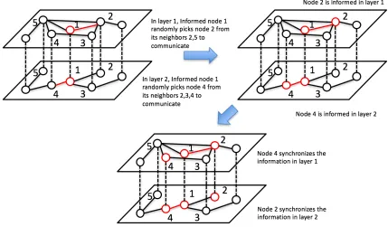
For the gossip algorithm in the single network, during the active time, each node contacts one of its neighbors independently and uniformly at random. During each meaningful contact (for which exactly one node has the piece of information1), the message is successfully delivered in either direction (through the “push” or “pull” operation). Specifically, for the push operation, the informed node randomly chooses a neighbor and attempts to pass the information, while for the pull opera-tion, the uninformed node randomly chooses a neighbor and attempts to grab the information. There are two key differences for information spreading in a multi-plex network: First, the message can be spread on multiple layers simultaneously. Second, when a node gets informed at one layer, it will automatically become in-formed at all other layers. While these two assumptions are somewhat idealistic, we will use them in this study to explore the maximum potential for information spreading in multiplex networks. In particular, we will consider the following gossip algorithm for a multiplex network: Before the gossip process, it is assumed that all duplicates of the same node are synchronized. During a gossip step, each node and its duplicates contact one of its neighbors (not necessarily the same in each layer) uniformly at random in all layers simultaneously. After each gossip step, the newly informed nodes (if exist) will broadcast the information to all their duplicates. The details are depicted in Fig. 2.1.
1While that the classic single piece information spreading problem is focused in this work, most of our
Figure 2.1: Gossip Algorithm in a Two-layer Multiplex Network
4. Information Spreading Time
The metric commonly used to measure the efficiency of gossip based information spreading is the information spreading time. Denote S(t) as the informed node set at the time t, with S(0) ={s}, for some arbitrary s ∈V. Two different spreading times are considered for the two time models.
• Standard Spreading Time: The standard information spreading time in a net-work G of size n, Tspr(G, γ), for some γ > 0, is defined as the stopping
time by which all nodes are informed with probability 1−O(n−γ) [32], i.e.,
Tspr(G, γ) = sup s∈V
inf{t : P r(St 6= V|S0 = {s}) ≤ O(n−γ)}. This is the metric used for the analysis of the synchronous gossip.
• Average Spreading Time: If given Tspr(G) as the stopping time by which all
nodes in the networkGare informed, the average spreading time is the average of Tspr(G) with respect to the random gossip process, as well as the random
2.2
Synchronous Gossip in Multiplex Networks
Analyzing the information spreading process is difficult even in a single network due to the heterogeneous network topology and random gossip processes. To the best of our knowledge, the tightest upper bound for the information spreading time in a general single network in literature is O(Φ−1·logn) [32, 33], where Φ is the corresponding graph conductance. The multiplex network structure introduces interconnections and interac-tions among layers, which further complicate the analysis. In this study, we slightly relax the problem and endeavor to find the information spreading time in a general multiplex network in an idealized setting. We are able to obtain a neat result in this setting (The-orem 2), which connects the information spreading time to a new metric for multiplex networks, multiplex conductance (Definition 5). In this section, the informed probabil-ity model is first introduced to facilitate the understanding of information spreading in multiplex networks. Then the corresponding information spreading time will be analyzed.
2.2.1
Informed Probability Model
In this part, the informed probability model is presented to offer some preliminary insights of information spreading in a multiplex network. In order to facilitate our analysis, the information spreading time is reformulated. First, theinformed probability is defined as:
Definition 1. The informed probability Pt,s(u), t ∈ N is defined as the probability that
node u becomes informed by roundt−1(right before round t) given that the source node is s.
Based on the above definition, the information spreading time is redefined:
Definition 2. Given the informed probability sets[Pt,s(u)]u∈V, t∈Ndefined for
informa-tion spreading in the network G= (V, E) of size n starting at node s, the corresponding information spreading time can be defined as
Tspr(G, γ, s) = inf{t : max
u∈V {(1−Pt,s(u))} ≤O(n
−γ−1)}, (2.1)
and the information spreading time of network G can be alternatively defined as
Tspr(G, γ) = sup s∈V
Remark 1. Given the information spreading timeTspr(G, γ), γ >0, (1−PTspr(G,γ)(u))≤
O(n−γ−1) holds for any source node s∈ V, and any other node u∈ V. The equivalence
between this new definition of information spreading time and the original one can be
shown by the following inequalities:
P r(not all nodes are inf ormed) =P r([
u∈V
node u is not inf ormed)
≤X
u∈V
P r(node u is not inf ormed)
=X
u∈V
(1−PTspr(γ)(u))≤n×O(n
−γ−1) = O(n−γ),
(2.3)
the first inequality is by union bound.
Therefore, the probability that all nodes are informed is at least 1−O(n−γ)after time
Tspr(G, γ), i.e., Tspr(G, γ) is the stopping time required for all nodes to be informed with
probability 1−O(n−γ).
Then, the following definition is needed for the following analysis:
Definition 3. Given a multiplex networkG={Gm ,(V, Em)}Mm=1, for each node u∈V,
dm(u) and N egm(u) are defined as the node degree and the neighbor set of u in layer m.
The maximum total node degree is then defined as ∆max = max u∈V (
M
P
m=1
dm(u)). The total
neighbor set N eg(u) of node u is defined as the set of all unique nodes connected to u in any layer, i.e., v ∈ N eg(u) if (u, v) ∈
M
S
m=1
Em. If v ∈ N eg(u), the link (u, v)’s existing
layer set is defined as L(u,v) = {α; (u, v) ∈ Eα},2 and the corresponding (u, v) link at
layer α is denoted as (u, v)α.
For an information spreading process in a graph G = (E, V) of size n with source
s ∈ V, given the informed probability set [Pt,s(u)]u∈V before round t, after gossiping at
round t the informed probability set [Pt+1,s(u)]u∈V is given by
Pt+1,s(u) =(1−(1−Pt,pull(u))(1−Pt,push(u)))
×(1−Pt,s(u)) +Pt,s(u),∀u∈V,
(2.4)
where Pt,pull(u) is the probability that node u pulls the information from its neighbor
nodes in round t, and Pt,push(u) is the probability that node u gets the information by
neighbors’ push operation in roundt. In the single network, nodeusuccessfully pulls the information from one of its neighbors when it contacts a node already informed, therefore the pull probability is given by
Pt,s,pull(u) =
X
v∈N eg(u) 1
d(u)Pt,s(v), (2.5) where d(u) is the degree of u.
Also, node u successfully gets pushed the information by its neighbors when any of its neighbors already informed contacts u, so the push probability is given by
Pt,s,push(u) = 1−
Y
v∈N eg(u)
1− 1
d(v)Pt,s(v)
. (2.6)
For a multiplex network G with M layers, node u successfully pulls the information when in any layers it successfully pulls the information. Therefore, the pull probability for an uninformed node u in network G is
Pt,pull(u) = 1− M
Y
m=1
1− X
v∈N egm(u) 1
dm(u)P t,s(v)
, (2.7)
For the push operation, in each round, node u gets pushed the information if any of its possible neighbor nodes already informed contacts it. For any v ∈ N eg(u), the probability thatv contacts nodeuis 1− Q
l∈L(u,v)
(1− 1
dl(v)). Therefore, the push probability for an uninformed node u in network G is
Pt,push(u) = 1−
Y
v∈N eg(u)
1− 1− Y
l∈L(u,v)
1− 1
dl(v)
!!
Pt,s(v)
!
. (2.8)
Remark 2. Due to the gossip nature, at each layer, an uninformed node only attempts
to pull the information from one neighbor, but may get pushed the information from
multiple neighbors. This accounts for the different expressions in Eq. (5) and Eq. (6)
when considering the overlapping edges across the layers.
of the multiplex network structure qualitatively, as shown in Theorem 1 below.
Theorem 1. Consider a multiplex network G(1) = {G(1) 1 , ..., G
(1)
M1}, and another mul-tiplex network G(2) built upon G(1) by adding additional M
2 −M1 layers, i.e., G(2) = {G(1)1 , ..., G(1)M
1, G
(2)
M1+1, ..., G
(2)
M2}, M2 > M1. Let Tspr(G
(1), γ) andT
spr(G(2), γ) be the
infor-mation spreading time for G(1) and G(2), respectively, then Tspr(G(1), γ)≥Tspr(G(2), γ).
Proof. The key point is to look into the informed probability Pt,s(u) for each node u.
From Eq. (2.7), the pull probability of nodeu in network G(1) is
P(1)t,s,pull(u) = 1− M1 Y
m=1
1− X
v∈N eg(1)m(u) 1
dm(u)P
(1)
t,s(v)
. (2.9)
Similarly for multiplex network G(2), the pull probability of node u is
P(2)t,s,pull(u) = 1− M2 Y
m=1
1− X
v∈N eg(2)m(u) 1
dm(u)P
(2)
t,s(v)
= 1−
M1 Y
m=1
1− X
v∈N eg(1)m(u) 1
dm(u)P
(2)
t,s(v)
×
M2 Y
m=M1+1
1− X
v∈N eg(2)m(u) 1
dm(u)P
(2)
t,s(v)
.
(2.10)
By Eq. (2.8), the push probabilities of node u in network G(1) and G(2) are
P(1)t,s,push(u)
= 1− Y
v∈N eg(1)(u)
1−1− Y
l∈L(1)(u,v)
1− 1
dl(v)
P(1)t,s(v)
!
,
P(2)t,s,push(u)
= 1− Y
v∈N eg(2)(u)
1−1− Y
l∈L(2)(u,v)
1− 1
dl(v)
P(2)t,s(v)
!
.
(2.11)
Eq. (2.7), P(1)t,pull(u) ≤ P(2)t,pull(u) since M2 > M1. Since G(2) is built upon G(1) by adding additional layers G(2)M1+1, ..., G(2)M2, then N eg(1)(u)⊂N eg(2)(u) and L(1)(u,v) ⊂L(2)(u,v),∀u, v ∈
V. Therefore, from Eq. (2.8), P(1)t,push(u)≤P(2)t,push(u). Finally,
P(1)t+1,s(u)
= (1−(1−P(1)t,s,pull(u))(1−P(1)t,s,push(u)))(1−P(1)t,s(u)) +P(1)t,s(u)
≤(1−(1−P(1)t,s,pull(u))(1−P(1)t,s,push(u)))(1−P(2)t,s(u)) +P(2)t,s(u)
≤(1−(1−P(2)t,s,pull(u))(1−P(2)t,s,push(u)))(1−P(2)t,s(u)) +P(2)t,s(u)
=P(2)t+1,s(u),∀u∈V.
(2.12)
Therefore, P(1)t,s(u) ≤ P(2)t,s(u),∀t ∈ Z, u, s ∈ V. Then the proof is finished up by contradiction: given source nodes, assume the information spreading times for networks
G(1) and G(2) are denoted by T1 and T2, respectively. Then by definition max
u {(1 − P(1)T1,s(u))} ≤O(n
−γ−1) and max
u {(1−P
(2)
T2,s(u))} ≤O(n
−γ−1). Also,
max
u {(1−P
(2)
T1,s(u))} ≤maxu {(1−P
(1)
T1,s(u))} ≤O(n
−γ−1). (2.13)
If T2 ≥ T1, then the above conclusion max
u {(1−P
(2)
T1,s(u))} ≤ O(n
−β−1) contradicts the definition T2 = inf{t: max
u {(1−P
(2)
t,s(u))} ≤O(n−β−1)}.
Therefore, for any given source node s∈V,Tspr(G(2), γ, s)≤Tspr(G(1), γ, s). Finally,
by Def. 2, Tspr(G(2), γ)≤Tspr(G(1), γ).
2.2.2
Idealized Information Spreading Time
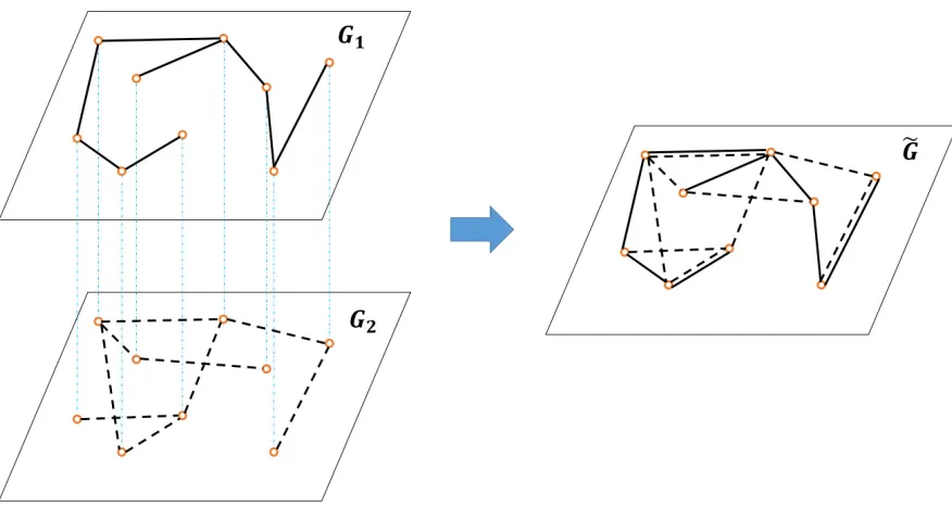
Figure 2.2: From Multiplex Network to Aggregated Multigraph
following so that the corresponding information spreading time can be analyzed, which serves as a good lower bound for the information spreading time of the original multiplex network. First, to handle the overlapping edges among layers, an aggregated multigraph representation for a multiplex network is constructed as follows.
Definition 4. Given a multiplex network G = {Gm , (V, Em)}Mm=1, the corresponding
aggregated multigraph G˜ = ( ˜V ,E˜) is defined such that V˜ = V and E˜ = ]M
m=1Em ,
{(u, v)α;u ∈ V, v ∈ N eg(u), α ∈ L(u,v)}, where ] stands for the non-unique set union,
i.e., the same links at different layers are all kept.
Remark 3. As shown in Fig. 2.2, an aggregated multigraph is obtained from the
corre-sponding multiplex network through a condensation process where the node set remains
the same and all links in all layers from the original multiplex network are kept. As a
result, multiple links can exist between the same pair of nodes u and v in the aggregated
multigraph if they are connected in multiple layers of the original multiplex network (e.g.,
(u, v) ∈ Eα,(u, v) ∈ Eβ, ...). In the aggregated multigraph G, these links are considered˜
To get around heterogeneous gossip at different layers, node u’s contacting proba-bility for each link (u, v)α is unified as P(u) = P((u, v)α) = min1
m∈{1,...,M}dm(u)
(denoted as link picking probability). This over-optimistic choice simplifies our analysis, while still providing a good lower bound as shown below.
The idealized setting is formed through a uniform gossip with link picking probability
P(u),∀u ∈ V, on the aggregated multigraph ˜G constructed above. The information spreading time in this idealized setting for an arbitrary multiplex network is quantified below.
Definition 5. The multiplex conductance Φmp of a multiplex network {Gm ,(V, Em)}Mm=1
is defined as
Φmp= min
S⊂V,volT(S)≤|E|T
M|cutT(S, V −S)| volT(S)
, (2.14)
where volT(S) =
M
P
m=1
volm(S), |E|T = M
P
m=1
|Em|, and |cutT(S, V −S)|=
M
P
m=1
|cutm(S, V −S)|.
volm(S)is the degree sum of all nodes in the node setSat layerm(volume), and|cutm(S, V−S)|
is the number of edges between node set S andV −S at layer m.
Remark 4. Multiplex conductance coincides with the original graph conductance [32]
when M = 1. Note that the factor of M is deliberately introduced to reflect the multiple information spreading processes in the multiplex network setting.
Theorem 2. For an M-layer multiplex network with n nodes, the information spreading
time in the idealized setting is at most 200(γ + 2)Φ−1
mp ·(logn + 12logM) rounds with
probability 1−O(n−γ), for some γ > 0, where Φmp is the multiplex conductance of this
multiplex network.
First, the following sequence of random variables solely related to the pull operation is introduced to facilitate our analysis. Let L1, L2, ... be a sequence of random variables with Li (i≥1) defined as follows. We distinguish two cases:
• IfvolT(Si−1)≤ |E|T, then by Definition 5,|cutT(Si−1, Ui−1)| ≥ M1 dΦmpvolT(Si−1)e ≥ 1
MdΦmpvolT(S0)e, where Ui−1 = V −Si−1 is the set of uninformed nodes at round
i−1. LetR =dΦmpvolT(S0)eandEibe an arbitrary subset of]Mm=1cutm(Si−1, Ui−1) consisting of M1R edges. Set Ei is (arbitrarily) fixed at the beginning of round
M ·min
m {dm(u)}. For each nodeu∈ Ui−1, let δi,u be the 0/1 random variable with
δi,u = 1 if and only if in round i node u pulls the information through some edge
inEi. Then, Li =Pu∈Ui−1(δi,uM ·minm {dm(u)}).
• IfvolT(Si−1)>|E|T, then Li =R.
Then, the following lemma is needed to prove Theorem 2:
Lemma 1. (a) E[P
k≤iLk] =iR and V ar(
P
k≤iLk)≤iR∆max, where
R=dΦmpvolT(S0)e. (2.15)
(b) If volT(S0)<∆max, then
P r(volT(Si)≥∆max)≥1/2, (2.16)
for i≥4∆max/(dΦmpvolT(S0)e).
(c) If ∆max ≤volT(S0)≤ |E|T then
P r(volT(Si)≥min{2volT(S0),|E|T + 1})≥1/2, (2.17)
for i≥4/Φmp.
(d) If volT(S0)>|E|T then
P r(volT(Ui)≤volT(U0)/2)≥1/2, (2.18)
for i≥6/Φmp.
Proof. The proof of Lemma 1 is provided in the appendix A.
Remark 5. The random variables Li are used to approximate the increment of volT(Si)
over the time. With the expectation and variance of the sum of random variables Li in
Lemma 1(a), different increasing speeds of volT(Si) are shown in Lemma 1(b), (c), and
(d), respectively, for three different stages ((d) actually shows the decreasing speed of its
Then, we can prove Theorem 2.
Proof for Theorem 2: When only the pull operation is considered, it can be seen from Lemma 1 that the total volume of the informed node set volT(Si) increases in different
ways in the three different stages. The information spreading analysis is then divided into three stages. In the first stage, by Lemma 1(b), if given volT(S0) < ∆max, after
at most d4∆max/(dΦmvolT(S0)e)e ≤ 5∆max/(dΦmvolT(S0)e) rounds, the total volume of the informed node set becomes at least ∆max with probability at least 1/2. Now,
divide the information spreading process in this stage into phases each comprised of 5∆max/(dΦmvolT(S0)e) rounds. A phase is considered successful if the total volume of the
informed node set at the end of that phase is at least ∆max. Therefore, in the firstd2βlnne
phases, the probability that none of them is successful is at most (1− 1/2)d2βlnne ≤
e−dβlnne=O(n−β). Therefore, with at mostd2βlnne ·5∆
max/(dΦmvolT(S0)e)≤3βlnn· 5∆max/(dΦmvolT(S0)e) rounds, the total volume of the informed node set hasvolT(St)≥
∆max with probability at least 1−O(n−β).
In the second stage, by Lemma 1(c), if ∆max ≤volT(S0)≤ |E|T, then with
probabil-ity at least 1/2, it takes at most d4/Φme rounds until the total volume of the informed
node set is increased to at least min{2volT(S0),|E|T + 1}. Similarly, divide the
infor-mation spreading process in this stage into phases of d4/Φme rounds each. A phase is
successful if the total volume of the informed node set at the end of the phase is at least min{2volT(Si),|E|T + 1}, whereSi is the set of informed nodes at the beginning of that
phase. Then, for any k, the probability that the k-th phase is successful is at least 1/2, regardless of the outcome of the previousk−1 phases. LetB(k,1/2) denote the binomial random variable for k trials each with success probability of 1/2. Then, by the Chernoff bound, the probability that fewer thanγ = log|E|T of the firstk = (2β+ 4)γ phases are
successful is at most
P r(B(k,1/2)≤γ)≤e−2(γ−k/2)2/k ≤e−βγ =O(n−β), (2.19)
since |E|T ≥ n−1. And since at most γ successful phases are required until the total
volume of the informed node set exceeds|E|T, it follows that with probability 1−O(n−β)
the number of rounds required is at most kd4/Φme ≤ k ·5/Φm ≤ (2β + 4)(2 logn+
logM)(5/Φm) as |E|T ≤M ·n2.
Finally, by Lemma 1(d), ifvolT(Si)>|E|T then, with probability at least 1/2, it takes
similar reasoning as before, we can show that once the total volume of informed nodes has exceeded|E|T, then (2β+4)(2 logn+logM)(7/Φm) rounds suffice to inform all nodes
with probability 1−O(n−β).
Combining all the above three cases and applying the union bound, we obtain that, with probability 1−O(n−β), all nodes get informed within 50(β+2)(logn+1
2logM)(Φ
−1
m +
∆max/(dΦmvolT(S0)e) rounds given any initial informed node set S0 when only the pull operation is considered.
Then let vmax be the node of maximum total degree ∆max (see Definition 3). From
above, the pull operation distributes the information from vmax to any other nodes in
50(β + 2)Φ−m1·(1 + ∆max
∆max)(logn + 1
2logM) = 100(β + 2)Φ
−1
m ·(logn + 12logM) rounds w.h.p. Then by Lemma 13 from [32] which shows the symmetry between the pull and push operation, the push operation can also spread tovmax the information started at an
arbitrary source node s in 100(β+ 2)Φ−1
m ·(logn+
1
2logM) rounds with the same high probability. Therefore, the push-pull operation can spread the information started at s
to all nodes in 200(β+ 2)Φ−1
m ·(logn+
1
2logM) rounds w.h.p.
Remark 6. By Theorem 2, we have shown that Θ(Φ−mp1 ·logn) is a good estimate for information spreading time in a general multiplex network in the idealized setting. It
becomes a true lower bound for the actual information spreading time when the layer number of multiplex networks is sufficiently large, as shown below.
Theorem 3. Given an M-layer multiplex network G = {Gm}Mm=1 with n nodes, there
always exists a constant cn>0 such that, when M > cn, Θ(Φ−mp1 ·logn)is a lower bound
of the actual information spreading time.
Proof. First, note that the calculated information spreading time Θ(Φ−1
mp · logn) is a decreasing function of M (|cutT(S,V−S)|
volT(S) = Ω( 1
n2) = Θ(1) when n is fixed), and it will go
to 0 as M goes to the infinity. Further note that the information spreading time of any scheme for any underlying network topology is lower bounded by some constant. Thus, there must exists a constant cn > 0 such that when M > cn, Θ(Φ−mp1 ·logn) is a lower bound of the actual information spreading time.
Θ(Φ−1
mp·logn) can still be a good lower bound for the actual information spreading time of a multiplex network. Two special cases of special interest are further discussed below.
Remark 7. If the single-layer bound is tight for information spreading time in every layer
of the given multiplex network (i.e., Tspr,i = Θ(Φ−i 1·logn), where Φi is the conductance
of the ith layer), then our bound is also tight in the corresponding aggregated multigraph
˜
G (i.e., T˜spr = Θ(Φ−mp1 ·logn)).
This is intuitively correct by the construction of the aggregated multigraph and the derivation of Theorem 2. In single networks, the above bound is known tight for many
graph models of interest. Prominent examples include complete graphs, random geometric
graphs (RGGs), and expander graphs (which include Preferential Attachment (PA) graphs
as a special case); their information spreading times areTC = Θ(logn), TRGG = Θ(logrn),
and TEX = Θ(logn), respectively, with the corresponding conductance given by ΦC = 12,
ΦRGG = Θ(r) (r is the radius of RGGs), and ΦEX = Θ(1).
Remark 8. If the single-layer bound is essentially tight for information spreading time
in every layer of the given multiplex network (i.e., Φ−1 = Θ(D(G)), where D(G) is the
diameter of the graph G, and Φ−1 =ω(logn)), then our bound is also essentially tight in
the corresponding aggregated multigraph G.˜
The information spreading time Tspr =O(Φ−1 ·logn) in the single network is
deter-mined by two factors: the inverse of graph conductanceΦ−1 and the logarithm of network
sizelogn. It is also known that a spreading algorithm in any graph needs at leastΩ(D(G))
rounds to finish. If Φ−1 = Θ(D(G)), it indicates that the inverse of graph conductance is on the same order as the graph diameter. The extra logn in the original bound is due to the distributed nature of the gossip algorithm, therefore it is essentially tight or gossip is
essentially effective in such graph structures. Ring graph is such an example, for which
the information spreading bound is essentially tight, since its conductance Φring = 2n and
diameter Dring = n2.
Many types of graphs as pointed out belong to the above two categories, except for star-like graphs, for which the conductance Φstar = 1 and the information spreading
time Tstar = 1. Therefore, we expect that a multiplex network comprised of component
layers constructed (or well modeled) by the above graphs will admit Θ(Φ−1
mp·logn) as a good lower bound for information spreading time3. In this case, the improvement in 3Note that different layers may have different structures (such as one PA layer coupled with one RGG
information spreading efficiency from a single network to a multiplex network can be orderly determined by PI = ΦΦmp.
2.2.3
Multiplex Conductance Evaluation and Performance
Im-provement
Our main result above, as a generalization and advance of the current art of the sin-gle network study, nicely encapsulates the gossip-based information spreading perfor-mance in a multiplex network into a metric, its multiplex conductance. In this part, the multiplex conductance is evaluated for some interesting multiplex networks to facilitate understanding.
As can be seen from Definition 5, the multiplex conductance is calculated through jointly minimizing the overall cut-volume ratio of the multiplex network. Evaluation of the single network conductance is in general a hard problem already, and existing re-sults are mainly obtained for graphs with certain nice properties and usually in the order form [12, 34]. The existence of multiple layers and interactions among layers further com-plicates the evaluation. Therefore, as a first work in this area, we will focus on evaluating some multiplex networks with special structures like ring graphs, which allow us to obtain some inspiring results. The study of the multiplex conductance for multiplex networks with other types of network topologies will be investigated in our future work. Based on the definition of multiplex conductance, two key factors contribute to higher information spreading efficiency in multiplex networks as compared to the single network: 1) avail-ability of multiple channelsM, and 2) larger contacting opportunities |cutT(S,V−S)|
volT(S) . There may be a common misconception that the best achievable improvement for information spreading in a multiplex network formed with similar-topology layers would be on the order of M. Our first example below dispels this misconception through an innovative design exploiting the second factor above.
Proposed Ring-Ring Multiplex Network
Figure 2.3: Proposed Ring-Ring Structure r = 4
first layer, each node with ID i connects with two nodes with IDs ((i+ 1) mod n) and ((i−1) mod n), which forms a normal ring structure. Next, assuming without loss of generality that n+ 1 is not a prime number, find out its factor r that is closet to √n. Then in the second layer, node with ID i is connected with two nodes with IDs ((i+r) mod n) and ((i−r) mod n) instead. Consider the right connection of each node, then in the second layer starts from node with ID 1, after n+1r such connections, it will reach the node with ID (1 + (n+ 1)) mod n which is 2. The same process repeats forn times, the right connections will reach back to node 1, therefore the second layer is guaranteed with a ring structure.
Then the multiplex conductance of this network structure is given by the following corollary:
Corollary 1. The multiplex conductance of the above proposed ring-ring multiplex
net-work is Φmp= 2 min
{r+1,(n+1)/r+1}
n .
Proof. The proof of Corollary 1 is provided in the appendix A.
100 1 102 103 104 105 50
100 150 200 250 300 350
Network Size
Efficiency Improvement
Simulation
Φm
Φ
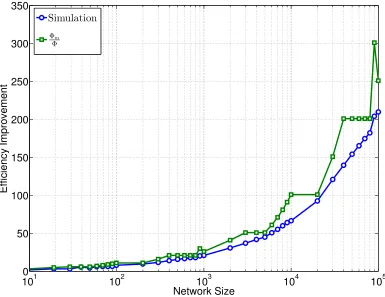
Figure 2.4: Efficiency Improvement for Proposed Ring-Ring
as shown in Fig. 2.4, the predicted information spreading efficiency improvement PI =
Φmp
Φ = min{r+ 1,(n+ 1)/r+ 1} is quite tight in this scenario.
Remark 9. The second layer of the proposed ring-ring structure dramatically increases
the size of cut (e.g., the size of the half-half cut is 2 in the original network but it be-comes 2r+ 2 in the proposed ring-ring structure) through the rewiring of nodes without increasing the set volume. This smart design leads to an information spreading efficiency
Different-Structure Multiplex Network
This example reveals increased contacting opportunities in a multiplex network from a new perspective. Note that multiplex networks don’t need to be constrained by construc-tion of similar-topology layers. Intuitively, a marriage of different structures can lead to a dramatic improvement in information spreading for the disadvantaged layer, as shown by the following two cases.
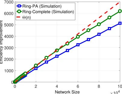
• Ring-Complete Coupling:If a ring graph is coupled with another complete graph to form a ring-complete multiplex network, the corresponding multiplex conductance may be computed as
Φmp= min
|S|≤n/2
2 2 +|S|(n− |S|)
2|S|+|S|(n−1) = Θ(1). (2.20) Then the performance improvement isPI = Θ(
Φmp
Φ ) = Θ(n).
• Ring-PA Coupling: Consider a PA graph with the parameter d, i.e., a new node connects to d existing nodes with probabilities proportional to their degrees, then the corresponding multiplex conductance of a ring-PA multiplex network is given by
Φmp= min
S∈V, volT(S)≤|E|T
2|cutr(S, V −S)|+|cutP A(S, V −S)|
volr(S) +volP A(S)
≥ min
S∈V, volT(S)≤|E|T
22 +|cutP A(S, V −S)| 2|S|+volP A(S)
≈ min
S∈V, volT(S)≤|E|T
2|cutP A(S, V −S)| 2|S|+volP A(S)
≥ min
S∈V, volT(S)≤|E|T
2 |cutP A(S, V −S)| 2|S|+d|S|+|cutP A(S, V −S)|
≥ 2α
2 +d+α = Θ(1),
(2.21)
0
2
4
6
8
10
Network Size
10
40
1000
2000
3000
4000
5000
6000
7000
Efficiency Improvement
Ring-PA (Simulation)
Ring-Complete (Simulation)
(n)
Identical-Graph Multiplex Network
Finally, the impact of layer numberM is explored, considering a special type of multiplex networks formed with M layers of identical topology. When M identical graphs having conductance Φ form a multiplex network, the overall multiplex conductance can be shown as
Φmp= min
S∈V,volT(S)≤|E|T
M· M · |cut(S, V −S)|
M ·vol(S) =MΦ.
(2.22)
Therefore, an improvement of orderM is expected for information spreading efficiency in this setting, which is generally an over-estimate, as the effect of link collision at different layers is ignored. This effect is most severe for the identical-layer structure, and can be partially corrected by considering the average meaningful contact for each node. For a node i with degree di in each layer, the average number of meaningful contacts in
each time slot after eliminating duplicate contacts is di(1−(1− d1i)M). Therefore, the
information spreading efficiency improvement for the whole network is upper bounded by ∆(1−(1− 1
∆)
M), where ∆ is the largest node degree across all layers in the network.
By dividing the single layer information spreading time by M and ∆(1−(1− 1 ∆)
M),
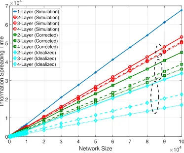
respectively, the idealized and corrected information spreading time can be calculated as shown by the bottom three grouped curves (with diamond markers) and middle three grouped curves (with square markers) in Fig. 2.6. When ∆ is small (like in the ring graph), this simple correction leads to an improvement as shown in Fig. 2.6. For multiplex networks constructed by independent layers, the over-estimation error is usually not a concern.
2.2.4
Layer Cost and Information Spreading Efficiency
In real life, the adoption of a new layer comes with an additional cost. In this section, the tradeoff between the improvement of information spreading efficiency and the additional layer cost is discussed. In particular, we will exam two types of cost below.4
• Network Cost for a User: The cost of additional layers from a user u’s aspect is 4The choices of cost in this paper mainly serve to facilitate relevant discussion. In practice, other
0 1 2 3 4 5 6 7 8 9 10
Network Size 104
0 1 2 3 4 5 6 7
Information Spreading Time
104
1-Layer (Simulation) 2-Layer (Simulation) 3-Layer (Simulation) 4-Layer (Simulation) 2-Layer (Corrected) 3-Layer (Corrected) 4-Layer (Corrected) 2-Layer (Idealized) 3-Layer (Idealized) 4-Layer (Idealized)
measured by the total degree of this node in all layers, i.e.,CM L(u) =PMm=1dm(u).
Therefore, the corresponding cost increase for the user u is CI,U(u) =
PM
m=1dm(u) d(u) , where d(u) is the node degree ofu in the initial single network.
• Network Cost for the Network Designer: Different from the user’s aspect, for a network designer, the cost of a new layer is better measured by the number of total edges of it. Then the cost increase for the network designer is CI,N =
PM m=1|Em|
|E| ,
where |E|is the number of total edges of the initial single network.
With the cost increment CI for each multiplex network, and the corresponding
in-formation spreading efficiency improvement PI, the reward-cost ratio can be defined as
RC = PI
CI. In the following, four related cases are examined to shed some light on the trade-off between performance improvement and cost:
1. From a ring graph to a two-identical-ring multiplex network: In this case, the information spreading efficiency improvement is 2. The cost increments for both the user and the network designer areCI,U =CI,N = 2. Then the reward-cost ratios
are RCU =RCN = 1.
2. From a ring graph to a two-layer ring-complete multiplex network: In this case, the performance improvement is PI = Θ(
Φmp
Φ ) = Θ(n) by Eq. (2.20). The cost increments for both the user and the network designer are CI,U =CI,N = n+12 .
Then the reward-cost ratios are RCU = RCN = Θ(1). Therefore, even though
the ring-complete coupling brings dramatic improvement in information spreading efficiency, the associated cost somewhat offsets its effectiveness.
3. From a ring graph to a two-layer ring-preferential-attachment (PA) mul-tiplex network: In this case, the performance improvement is PI = Θ(n) by Eq.
(2.21). But the cost increment is now different for the user and network designer, since the cost increments are different for different nodes due to network irregularity. Both the maximum cost increment Cmax
I,U and average cost incrementCI,Uave are
con-sidered for the user. Since the largest node degree in the PA network withn nodes grows as Θ(√n) [35], the maximum cost increment isCmax
I,U = Θ(
√
n). However, the average node degree for the PA network is 2d. Then the average cost increment is
0
2
4
6
8
10
x 10
40
200
400
600
800
1000
1200
1400
1600
1800
Network Size
Reward−Cost Ratio
Ring−PA (Average)
Ring−Ring (Proposed)
Ring−PA (Minimum)
Ring−Ring (Identical)
Ring−Complete
0
2
4
6
8
10
x 10
40
20
40
60
80
100
120
Network Size
Reward−Cost Ratio
Ring-Ring (Proposed)
Θ
1(
√
n
)
Ring-PA (Minimum)
Θ
2(
√
n
)
Ring-Ring (Identical)
Ring-Complete
network designer, the cost increment is CI,N = d+ 1, and the reward-cost ratio is
RCN = Θ(n). Clearly, the ring-PA coupling is much more effective as compared to
the ring-complete coupling when the layer cost is explicitly considered.
4. From a ring graphto the ring-ring structure proposed in 2.2.3: It has been shown that the efficiency improvement is PI = min{r + 1,(n + 1)/r + 1}. The
cost increments for both the user and the network designer are CI,U = CI,N = 2,
then the reward-cost ratios are RCU =RCN = min{r+1,(n2+1)/r+1}, which is close to
Θ(√n) in most scenarios.
Remark 10. Figs. 2.7 and 2.8 simulate the actual reward-cost ratios from the user’s
perspective, while Figs. 2.9 and 2.10 present the results from the network designer’s
view-point. From both the discussion above and simulations, it can be seen that, overall
speak-ing, the ring-PA coupling is the most effective multiplex structure as far as information
spreading is concerned. Since PA graph is a popular model for social platforms, this
re-sult partially reveals the beneficial impact of utilizing social networks for information
distribution.
On the other hand, the preferential attachment design is much more complicated as compared with our proposed ring-ring structure. Therefore, as far as the overall network
design is concerned (instead of utilizing existing network structures), our proposed
struc-ture provides the insight that a careful planning of the new layer strucstruc-ture can greatly
improve the overall efficiency for information spreading without incurring much
addi-tional cost.
The goal of this section is to study the benefit of facilitating the information spreading
in multiplex networks through additional layers. We picked three different topologies, ring
graph, complete graph, and PA graph, as candidates for each layer of multiplex networks.
The complete graph represents the idealized single network structure which serves as a base line compared to any other topologies. The PA graph, which has a large amount of edges, a
very small diameter, and is well-connected, is chosen as an extreme but realizable topology
for a single network. In reality, it corresponds to the social network that greatly speeds
up the information spreading process on top of the traditional communication networks.
Despite of the effectiveness in spreading information, its existence requires a huge amount
of management and computation resource. The ring network, which has a much smaller
number of edges, a large diameter, and is very poor-connected, is chosen as another
0
2
4
6
8
10
x 10
40
200
400
600
800
1000
1200
1400
1600
1800
Network Size
Reward−Cost Ratio
Ring−PA
Ring−Ring (Proposed)
Ring−Ring (Identical)
Ring−Complete
0
2
4
6
8
10
x 10
40
20
40
60
80
100
120
Network Size
Reward−Cost Ratio
Ring-Ring (Proposed)
Θ
1(
√
n
)
Ring-PA (Minimum)
Θ
2(
√
n
)
Ring-Ring (Identical)
Ring-Complete
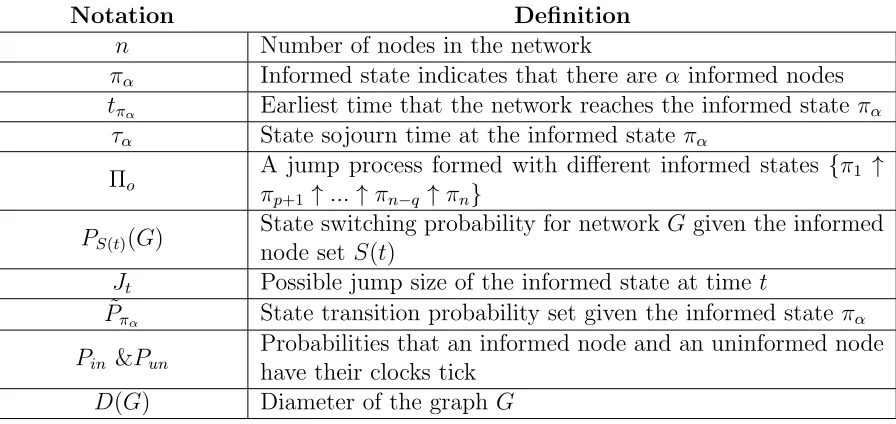
Table 2.1: Important Notations with Definitions
Notation Definition
n Number of nodes in the network
πα Informed state indicates that there are α informed nodes
tπα Earliest time that the network reaches the informed state πα
τα State sojourn time at the informed state πα
Πo
A jump process formed with different informed states {π1 ↑
πp+1↑...↑πn−q↑πn}
PS(t)(G)
State switching probability for networkG given the informed node set S(t)
Jt Possible jump size of the informed state at time t
˜
Pπα State transition probability set given the informed state πα
Pin &Pun
Probabilities that an informed node and an uninformed node have their clocks tick
D(G) Diameter of the graph G
to the type of networks that a small group of people want to build to facilitate their own information spreading with a limited budget (small number of edges) and the real spatial
constraint (poor-connected) on top of the existing social and communication networks.
2.3
Asynchronous Gossip in Multiplex Networks
Our main results are summarized below as Theorems 4-8. The impacts of layer number, layer similarity, and average node degree on the efficiency of information spreading are presented in Theorems 4-7, respectively, with the assumptions that all networks are con-nected. The multiplex network connectivity is discussed in Theorems 8 and 9. Important notations used in this part are listed in Table. 2.1.
2.3.1
Qualitative Spreading Time Comparison
One key idea in our following analysis is to describe the whole information spreading process as a jumping process: {π1 ↑ πα ↑ ... ↑ πn−β ↑ πn}, where πα is referred to
as the informed state, indicating that there are α informed nodes in the network (not counting duplicates in different layers for a multiplex network). In a network of size
asynchronous time model, state transition can only happen at timesZs, s∈N when the clock of one node ticks and it exchanges information with one of its neighbors. Define
tπα = inf{t:|S(t)|=α} as the earliest time that the network reaches the informed state
πα, andτα = inf{t:|S(tπα +t)|> α} as the state sojourn time atπα. Due to the nature of the gossip mechanism, {τα}nα−=11 are independent from each other. It is also assumed that the node communication time is negligible. For a single network, the jump size J
is always 1 between adjacent informed states. Thus, E(Tspr) = n−1
P
i=1E
(τi). However, for a
multiplex network ofM layers,J ranges from 1 toM due to possibly different topologies in these layers and the synchronization of messages among the duplicates of the same node after each gossip step. Therefore, information spreading in a multiplex network can lead to different jump processes: Πo = {π1 ↑ πp+1, ..., πn−q ↑ πn},1 ≤ p, q ≤ M.
Thus, for a given Πo, we haveE(Tspr|Πo) =
P
πl∈Πo
E(τl), andE(Tspr) =E(E(Tspr|Πo)). Our
first main result below verifies the intuition that two are better than one. In particular, if we add a layer of network with arbitrary degree distribution to an existing one, the information spreading performance always improves. To prove this result, we need the following definition and Lemma 2 which compares the expected state sojourn times for single networks and two-layer multiplex networks at the same informed state.
Definition 6. For a given single network G, the state switching probability PS(t)(G) is
defined as the probability that a new node in the network G will be informed given the
informed node set S(t).
Lemma 2. Given a single random network G1 with degree distribution P(k), and a
two-layer random multiplex network G2 = (G21, G22) with the degree distribution P(k) and ˆ
P(k), respectively, if networksG1 andG2 are in the same informed stateπα, α∈[1, n−1],
the expected state sojourn times for these two networks admit E(τα(1))≥E(τα(2)).
Proof. First, for a given single network G1 with degree distribution P(k), given an in-formed node set S(t) such that |S(t)| = α, the state switching probability PS(t)(G1) is defined as the probability that a new node in the networkG1 will be informed given the informed node set S(t), which will be simplified as PS(1)(t). According to the gossip mech-anism, the state sojourn time τS(t)(G1) =
Ng
P
i=1
Ti, where {Ti} are time intervals between