ABSTRACT
SKAU, ERIK WEST. Relaxations to Sparse Optimization Problems and Applications. (Under the direction of Agnes Szanto and Hamid Krim.)
Parsimony is a fundamental property that is applied to many characteristics in a variety of fields. Of particular interest are optimization problems that apply rank, dimensionality, or support in a parsimonious manner. In this thesis we study some optimization problems and their relaxations, and focus on properties and qualities of the solutions of these problems.
The Gramian tensor decomposition problem attempts to decompose a symmetric tensor as a sum of rank one tensors. We approach the Gramian tensor decomposition problem with a relaxation to a semidefinite program. We study conditions which ensure that the solution of the relaxed semidefinite problem gives the minimal Gramian rank decomposition.
Sparse representations with learned dictionaries are one of the leading image modeling tech-niques for image restoration. When learning these dictionaries from a set of training images, the sparsity parameter of the dictionary learning algorithm strongly influences the content of the dic-tionary atoms. We describe geometrically the content of trained dictionaries and how it changes with the sparsity parameter. We use statistical analysis to characterize how the different content is used in sparse representations. Finally, a method to control the structure of the dictionaries is demonstrated, allowing us to learn a dictionary which can later be tailored for specific applications.
Variations of dictionary learning can be broadly applied to a variety of applications. We explore a pansharpening problem with a triple factorization variant of coupled dictionary learning. Another application of dictionary learning is computer vision. Computer vision relies heavily on object detection, which we explore with a hierarchical convolutional dictionary learning model.
© Copyright 2017 by Erik West Skau
Relaxations to Sparse Optimization Problems and Applications
by Erik West Skau
A dissertation submitted to the Graduate Faculty of North Carolina State University
in partial fulfillment of the requirements for the Degree of
Doctor of Philosophy
Applied Mathematics
Raleigh, North Carolina
2017
APPROVED BY:
Seth Sullivant Dávid Papp
Agnes Szanto
Co-chair of Advisory Committee
Hamid Krim
DEDICATION
BIOGRAPHY
Erik Skau received B.S. degrees in Applied Mathematics as well as Physics (2010) in Raleigh, NC at North Carolina State University. In graduate school under the direction of Dr. Agnes Szanto and Dr. Hamid Krim, Erik pursued an applied mathematics degree.
ACKNOWLEDGEMENTS
I would first like to thank my advisors Dr. Agnes Szanto and Dr. Hamid Krim for their tremendous help and support in this process. They provided invaluable advice and guidance for both academic problems and with life’s challenges. Additionally I would like to thank the rest of my committee, Dr. Edge Lobotan, Dr. Dávid Papp, and Dr. Seth Sullivant for both their suggestions and patience during my graduate career.
Additionally, I would like to thank Dr. Greg Bleckerham, Dr. Liyi Dai, Dr. Lek-Heng Lim, Dr. Bernard Mourrain, Dr. Jim Renegar, Dr. Michael Singer, and Dr. Brendt Wohlberg for their useful suggestions related to various sections of this thesis.
TABLE OF CONTENTS
LIST OF TABLES . . . vii
LIST OF FIGURES. . . .viii
Chapter 1 INTRODUCTION . . . 1
1.1 Outline . . . 1
Chapter 2 Sparsity and Opt. Background . . . 3
2.1 Principle of Sparsity . . . 3
2.1.1 Characterizing Sparsity with Norms . . . 3
2.2 Opt. and Relaxations . . . 5
Chapter 3 GRAMIAN TENSOR DECOMP. . . . 7
3.1 Introduction . . . 7
3.1.1 Background . . . 7
3.1.2 Related Work . . . 9
3.2 Preliminaries . . . 11
3.3 Relaxation and Dual Problem . . . 15
3.4 Certificate of Optimality . . . 17
3.5 Sufficient Cond. for Optimality . . . 20
3.6 Cases When Md+1 is Never Optimal . . . 25
3.7 Uncertain Cases . . . 26
3.7.1 Future Work . . . 26
3.8 Conclusion . . . 27
Chapter 4 SPARSITY PARAM. SELECTION IN D.L. . . . 29
4.1 Introduction . . . 29
4.1.1 Sparse Representation and Dictionary Learning Background . . . 29
4.1.2 Image Restoration . . . 32
4.2 Sparsity Parameter . . . 33
4.2.1 Geometric Interpretation . . . 35
4.2.2 Geometric Effect of Sparsity Parameter on Synthetic Data . . . 36
4.2.3 Geometric Effect of Sparsity Parameter on Image Patches . . . 38
4.2.4 Single Step Update . . . 41
4.3 Proposed Modification . . . 44
4.3.1 Proposed Modification on Synthetic Data . . . 45
4.3.2 Proposed Modification on Image Patches . . . 46
4.4 Conclusion . . . 47
Chapter 5 VARIATIONS OF D.L. AND APPS.. . . 50
5.1 Pansharpening via Triple Fact. D.L. . . 50
5.1.1 Introduction . . . 50
5.1.3 Related Works and Our Contribution . . . 51
5.1.4 Problem Formulation . . . 52
5.1.5 Algorithm . . . 54
5.1.6 Training Procedure . . . 54
5.1.7 Validation Procedure . . . 54
5.1.8 Moffett Dataset Results . . . 54
5.1.9 Conclusions . . . 55
5.2 Hierarchical Conv. D.L. . . 55
5.2.1 Introduction . . . 55
5.2.2 Convolutional Dictionary Learning and Max Pooling Background . . . 56
5.2.3 Hierarchical Convolutional Dictionary Learning . . . 57
5.2.4 Results and Discussion . . . 57
5.2.5 Future Work . . . 58
5.2.6 Conclusion . . . 60
Chapter 6 FUSING HETEROGENEOUS DATA . . . 62
6.1 Introduction . . . 62
6.2 Related works . . . 64
6.3 Prob. Statement and Formulation . . . 65
6.3.1 Weather-related Data: Boulder Colorado . . . 65
6.3.2 Problem Formulation . . . 68
6.4 Algorithmic Fusion Solution . . . 70
6.4.1 A Maximum Likelihood Equivalence . . . 70
6.5 Results and Discussion . . . 71
6.5.1 Fusing Unstructured Data: Tweets . . . 71
6.5.2 Unstructured Data: Manual Classification . . . 71
6.5.3 Unstructured Data: Location Correction . . . 72
6.5.4 Structured Data: SFHA . . . 75
6.5.5 Feature Generation . . . 76
6.5.6 Robustness to Malicious Information . . . 77
6.6 Conclusion . . . 79
Chapter 7 CONCLUSION. . . 82
LIST OF TABLES
Table 4.1 Usage statistics of two different classes of atoms trained using lasso with MOD. 39 Table 4.2 Usage statistics of two different classes of atoms trained using OMP with K-SVD. 40 Table 4.3 Statistics of minimal angles after a singleX andD update. . . 44 Table 4.4 Usage statistics of a dictionary trained with a variety of effective regularizations. 46
Table 5.1 Comparison of methods. . . 55
LIST OF FIGURES
Figure 2.1 Level curves for a variety of norm functions. . . 4
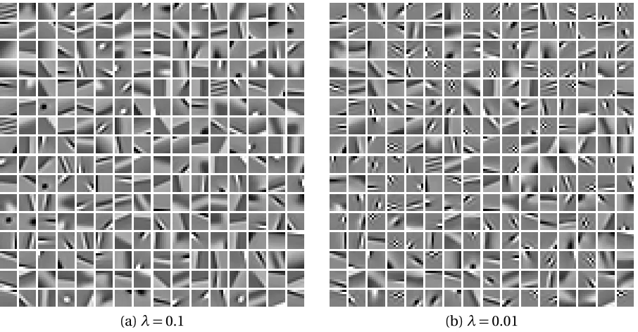
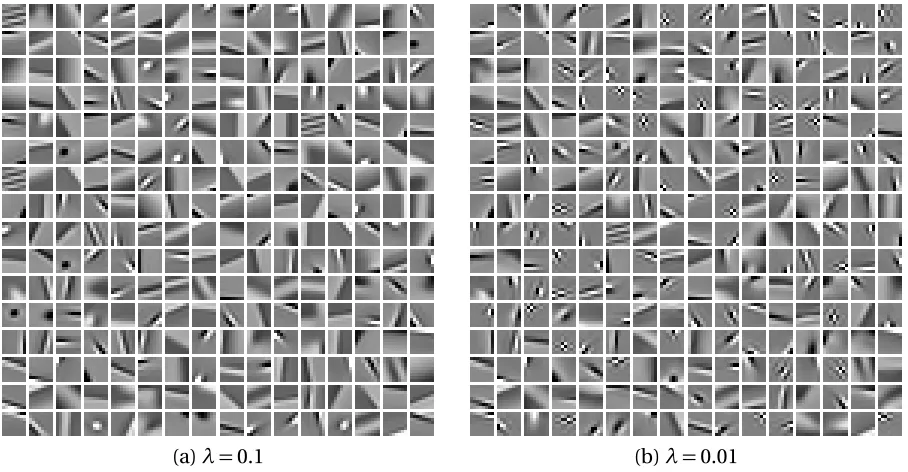
Figure 4.1 Dictionaries trained on natural image patches data using lasso with MOD. . . 34
Figure 4.2 Denoising performance of two dictionaries at a variety of noise levels and regularizations. . . 35
Figure 4.3 Example dictionaries to represent a 2-dimensional affine region. . . 36
Figure 4.4 Dictionaries trained on synthetic data using lasso with MOD. . . 37
Figure 4.5 Dictionaries trained on synthetic data using OMP with K-SVD. . . 38
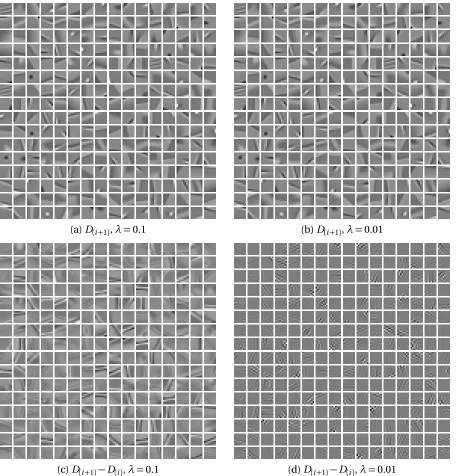
Figure 4.6 Dictionaries trained on natural image patches data using lasso with MOD. . . 39
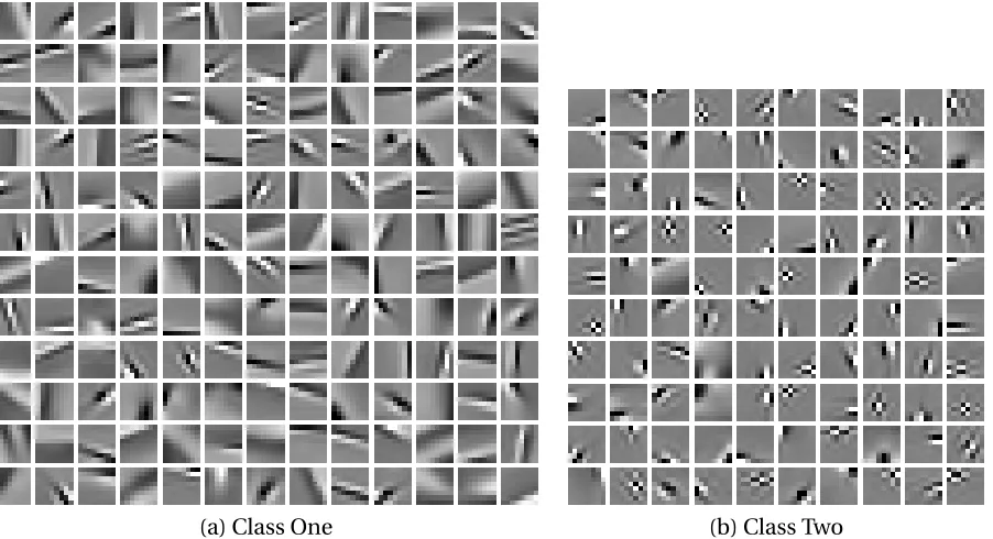
Figure 4.7 Dictionary atoms trained withλ=.01 regularization using lasso with MOD and visually split into two classes. . . 40
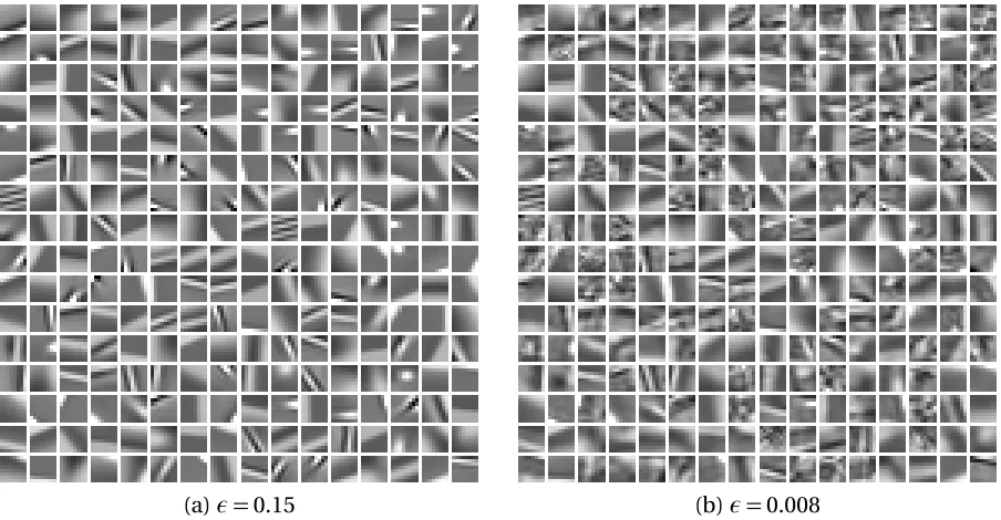
Figure 4.8 Dictionaries trained on natural image patches data using OMP with K-SVD. . 41
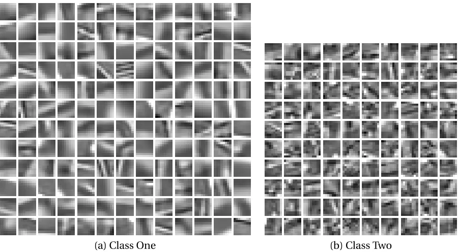
Figure 4.9 Dictionary atoms trained withλ=.01 regularization using OMP with K-SVD, visually split into two classes. . . 42
Figure 4.10 Single update step from learned dictionary with different regularizations, and the differences in steps. . . 43
Figure 4.11 Dictionary trained on synthetic data by (4.4) with effective regularizations of 0.009, 0.009, and 0.012. . . 45
Figure 4.12 Dictionary, D3, trained on natural image patches with different sparsity weights on different atoms using formulation 4.4. . . 47
Figure 4.13 Comparison of dictionaries at a variety of noise levels and regularizations. . . 48
Figure 5.1 Sample dictionary atoms transformed to the reference image space. . . 52
Figure 5.2 Sample dictionary atoms transformed to the degraded input image space. . . 52
Figure 5.3 Some sample reference and degraded images to be sharpened from Moffett data set . . . 53
Figure 5.4 Dictionary of 8 by 8 filters trained on faces from the Extended Yale Face Database B. . . 58
Figure 5.5 Convolution of two hierarchies of dictionaries trained on the Extended Yale Face Database B. . . 59
Figure 5.6 Reconstruction of the high pass training images where the contribution of the hierarchical dictionary filter corresponding to an eye is portrayed in red. . 60
Figure 5.7 Synthetic image comprised of square perimeters. . . 60
Figure 5.8 Hierarchical dictionaries trained on a synthetic image of squares. . . 61
Figure 6.1 Data from the 2013 Boulder, CO flood. . . 66
Figure 6.2 The results of a maximum entropy estimation using the tweet empirical dis-tribution and the landsat photos taken after the flood. . . 72
Figure 6.3 An overlay of tweets classified as indicative of flooding. . . 73
Figure 6.4 The results of a maximum entropy estimation using the manually classified tweets and the landsat photos taken after the flood. . . 74
Figure 6.6 The results of a maximum entropy estimation using the nearest neighbors relocated tweets and the landsat photos taken after the flood. . . 76 Figure 6.7 The results of a maximum entropy estimation using the SFHA and the landsat
photos taken after the flood. . . 77 Figure 6.8 The sparse representations after dictionary learning. . . 78 Figure 6.9 ROC curve comparison of dictionary learned estimation and the estimation
from the features the dictionary was trained on. . . 78 Figure 6.10 Maximum entropy estimation with mixture distributions . . . 80 Figure 6.11 ROC curves comparing different mixture levels of the empirical tweet and the
CHAPTER
1
INTRODUCTION
Parsimony is a concept fundamental to many problems and applications. Parsimonious characteris-tics can emerge in a wide range of things from order, support, rank, and dimension. In practice one often formulates optimization problems to encourage parsimony, or strives for sparsity in some characteristic.
Optimization problems with a sparsity characteristic are notoriously hard to solve. Fortunately, relaxations of these problems often provide surrogate problems that are much more tractable. These tractable problem solutions are then taken as approximations to the ideal solutions. This relaxation procedure brings into question exactly how close the relaxed solution is to the ideal solution.
In this dissertation, we consider varying forms of relaxations to parsimonious optimization problems and applications. In some instances we consider properties of the original and not re-laxed problems. In other instances, we consider the effect of sparsity on our models and propose modifications to the problems to yield a more desirable solution.
1.1
Outline
relaxation these non-convex problems can be replaced with convex surrogates. Some of these relaxations have properties suitable for algorithms to solve efficiently.
In Chapter 3 we look at the Gramian tensor decomposition problem. The tensor decomposition problem is formulated as a rank minimization optimization problem, which is relaxed to a nuclear norm minimization problem. Our interest in this research is to find cases where the relaxed nuclear norm solution is also of minimal rank. We then provide some specific cases where the optimal nuclear norm solution is also minimal rank and discuss the intricacy of the problem in other cases.
Chapter 4 introduces dictionary learning and some popular methods to solve dictionary learn-ing problems. Dictionary learnlearn-ing has a range of applications in image restoration problems. We consider a geometric interpretation of dictionary learning and the role of sparsity in the dictionary learning model. We present some of these applications, and proposed modifications to dictionary learning.
Chapter 5 explores two applications using variations of dictionary learning. In this chapter, coupled dictionary learning is reformulated to include an additional factorization and is applied to a pansharpening problem. We also develop a proof of concept for a hierarchical convolutional dictionary learning method to construct more complex dictionary filters.
In Chapter 6 we consider a data fusion problem for hazard extent estimation. We explore the suitability of using social media data to estimate the extent of inundated areas using a regularized maximum entropy model. We compare the effectiveness of using social media data against expert knowledge and discuss the filtering required of the social media.
CHAPTER
2
SPARSITY AND OPTIMIZATION
BACKGROUND
This chapter provides some of the main concepts and mathematical tools used to understand and formulate applicable optimization problems.
2.1
Principle of Sparsity
In a variety of fields, data is effectively of low order, support, rank, or dimension. In the last several decades, optimization problems applying these characteristics have become a widely used tool for a variety of applications[99, 126, 140]. The underlying principle of parsimony is common to all of these applications, simply applied to different characteristics. In this chapter we review some of the mathematical formulations of these notions for their incorporation into optimization problems. Since these notions are closely related, we concentrate on the notion of support size, or sparsity, and describe the relation between support and the other notions.
2.1.1 Characterizing Sparsity with Norms
Definition 2.1.1. Given an n dimensional vectorxin Euclidean space,Rn, the p -norm is defined for p>0as
kxkp=
n X
i=1
|xi|p
p1 .
Whenp=2, it is called the`2norm, or Euclidean norm, and simplifies to
kxk2=
v u t
n
X
i=1
xi2.
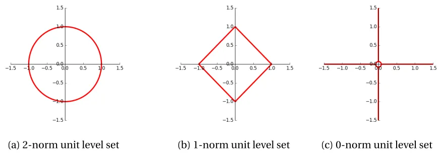
The 2-norm is a convex function. A depiction of the`2unit ball can be seen in Figure 2.1 (a).
Whenp=1 the norm is called the`1norm, taxicab norm, or Manhattan norm as it is
represen-tative of how a taxi measures distance in city blocks. The`1norm simplifies to
kxk1=
n
X
x=1
|xi|
and is a convex function. A depiction of the`1unit ball can be seen in Figure 2.1 (b).
(a) 2-norm unit level set (b) 1-norm unit level set (c) 0-norm unit level set
Figure 2.1Level curves for a variety of norm functions.
The limit asp approaches 0 relates to the so called 0-norm which is not actually a norm, but measures the number of nonzero elements in a vector, or the size of its support. The 0-norm is denoted
kxk0=lim
p→0kxk
p p=plim→0
X |xi|p,
defined as the number of zero-valued elements divided by the total number of elements, or in the case of ourndimensional vector,n−kxk0
n . These mathematical functions can be used to characterize
the fundamental properties that are pervasive in so many fields.
2.2
Optimization and Relaxations
Optimization problems are used to search a space for the best element with regard to some crite-rion. Within the field of optimization there are two principle categories, convex and non-convex optimizations. Convex optimization problems, which entail optimizing a convex function over a convex set, are in many senses much easier than non-convex optimization problems. The tools for non-convex problems include heuristic local methods that fail to guarantee global optimality such as gradient descent, and exact methods such as branch-and-bound that take exponential effort. Convex optimization problems, on the other hand, have the distinct benefit that local solutions are also globally optimal. This allows for global optimality with relatively quick gradient based methods.
Due to the relative ease of solving convex problems, non-convex problems are often approxi-mated with a convex surrogate[16, 64, 98]. In applications where some characteristic should be used parsimoniously, it is natural to integrate this into the optimization problems. For instance, when sparsity is a desirable characteristic, it makes sense to insert this into the objective function. Though the 0-norm perfectly characterizes sparsity, the fundamental quality we often wish to promote, its non-convexity poses significant challenges in optimization. Consider the example minimization problem
arg min
x k
xk0
subject to 1 2 x1 x2 =2 (2.1)
with two optimal solutions ofx= [0, 1]T andx= [2, 0]T. To find these solutions we must take a com-binatorial approach, restricting the support of the vectorxand solving the system. In such a small example this is not problematic, but as the problem size grows this quickly becomes computationally infeasible.
The convex relaxation of (2.1) to
arg min
x kxk1
subject to 1 2 x1 x2 =2 (2.2)
relaxation is one of the solutions to the original non-convex problem, while the other solution is lost in the relaxation. This type of relaxation technique is a powerful tool with both heuristic support [127, 140, 141]and theoretical merit[48, 49, 51, 143].
Another parsimonious characteristic in a significant number of applications is rank. The rank of the matrix,A, can be calculated from its singular values and the 0-norm.
Definition 2.2.1. Given an n by m matrix A with singular valuesσ=σ1, . . . ,σmin(m,n)
the rank can be defined as
rank(A) =kσk0
In rank minimization problems, one searches the feasible space for the lowest rank solution which also requires a combinatorial approach. To approximate a solution one can replace rank with nuclear norm.
Definition 2.2.2. Given an n by m matrix A with singular valuesσ=σ1, . . . ,σmin(m,n)
the nuclear
norm of A, denotedkAk∗, can be defined as
kAk∗=trace(
p
A∗A) =kσk1
This provides a computationally feasible objective function first introduced in[54]that can be used to approximate minimal rank solutions in many instances[98].
CHAPTER
3
GRAMIAN TENSOR DECOMPOSITION
3.1
Introduction
In this chapter we examine a tensor decomposition problem, posed as a rank minimization problem. We study the relaxation of the problem and consider cases when the relaxed solution is a solution to the original problem. In some instances of tensor rank and order, we prove generically that the solution to the relaxation will be optimal in the original. In other cases we present interesting examples and approaches that demonstrate the complexities of this problem.
3.1.1 Background
LetA ∈F(n+1)×···×(n+1)be aD-way, or orderD, symmetric tensor over a fieldFof size(n+1)×· · ·×(n+1) (D-times). LetR:=F[x1, . . . ,xn]and letRD denote the set of polynomials of degree at mostDinR.
Then we can associate toA a polynomial
p= X
β∈Nn,|β|≤D
D
D− |β|,β1, . . . ,βn
pβxβ∈RD (3.1)
by simply multiplyingA by the vector[1,x1, . . . ,xn]from all theD directions. This gives a bijection
between symmetricD-way tensors overFand polynomials inRD.
Definition 3.1.1. We say thatA ∈F(n+1)×···×(n+1)hassymmetric rankr if there exist distinctv1=
(v1,0,v1,1, . . . ,v1,n), . . . ,vr= (vr,0,vr,1, . . . ,vr,n)∈Fn+1with coordinates from the algebraic closureFof F, andλ1, . . . ,λr∈F/{0}such that r is minimum and
A =
r
X
t=1
λtvt⊗D:= r
X
t=1
λt
vt,i1· · ·vt,iD n
i1,...,iD=0. (3.2) Equivalently, we say that p∈RDhasrankr if r is minimal and
p=
r
X
t=1
λtLDvt, (3.3)
where Lvt(x1, . . . ,xn):=vt,0+vt,1x1+· · ·+vt,nxnis the linear form associated tovt = (vt,0,vt,1, . . . ,vt,n) for t =1, . . . ,r . The expressions in (3.2) or (3.3) are called therankr symmetric decompositionsofA and p , respectively.
There are different, non-equivalent notions of tensor rank in the literature, such as the multilinear rank or non-symmetric rank, etc. (see[32]). Also, one can define the symmetric rank over non-algebraically closed fields, which unlike for matrices, may differ from the above defined symmetric rank for tensors of order>2. If the fieldFis the set of real numbers and the orderD=2d is even, we can define theGramian rankas follows:
Definition 3.1.2. LetA ∈R(n+1)×···×(n+1)be a real symmetric tensor of order2d and p ∈R2dbe the
corresponding real polynomial. We say thatA and p isGramianwithGramian rankr if there exist
distinctv1= (v1,0,v1,1, . . . ,v1,n), . . . ,vr = (vr,0,vr,1, . . . ,vr,n)∈Rn+1andλ1, . . . ,λr ∈R>0positive real
numbers such that r is minimal and (3.2) or (3.3) holds. The decompositions in (3.2) and (3.3) are called theGramian decompositionsofA and p , respectively.
In this chapter we consider the problem of finding the Gramian rank and decomposition for a real symmetric tensor of order 2d, or equivalently, for a polynomial of degree 2d. Note that not all polynomials of degree 2d are Gramian, in particular, Gramian polynomials are a subset of sum of square polynomials. Hillar and Lim in[69]proved that deciding whether a tensor/polynomial is Gramian is NP-hard even ford=2. Also note that even if a tensor is Gramian, its Gramian rank may be much higher than its symmetric rank.
The main results of this Chapter are as follows:
• We give a meaningful semidefinite relaxation of the problem of finding the Gramian rank and decomposition of a polynomialp∈R2d, assuming that its Gramian rank is sufficiently small.
The relaxation becomes a matrix completion problem of moment matrices with minimal trace.
• We simplify and interpret the condition that a given moment matrix is the optimum of our relaxed semidefinite program, using special properties of the dual of the semidefinite program.
• We analyze special cases when we can guarantee that a given moment matrix is the optimum of the relaxed semidefinite program. In these special cases we point to a connection to the theory of the regularity index of overdetermined polynomial systems. Using this theory we list triples (n,d,r)where we can prove that the optimum of the semidefinite relaxation corresponds to the Gramian decomposition of rankr of a polynomial of degree 2d innvariables.
3.1.2 Related Work
Motivation for looking at the tensor decomposition problem comes from its broad application areas. The earliest results on tensor decomposition were applications in mathematical physics ([70, 71]); psychometrics ([24, 25, 67, 145, 146]); algebraic complexity theory ([72, 81, 83, 85, 86, 138]); and in chemometrics ([6, 61, 135]). In higher order statistics, moments and cumulants are intrinsically tensors (cf.[109]). Symmetric tensor decomposition is proven to be useful inblind source separation
techniques, which are capable of identifying a linear statistical model only from its outputs (cf. [33]). These blind identification techniques in turn are very popular in numerous applications, including telecommunication ([2, 66, 130]); radar ([26]); biomedical engineering ([41]); image and signal processing ([42, 63]) just to name a few. An excellent survey of more recent applications of tensor methods can be found in[69].
exist as the set of rankr tensors is not closed[132]
As we will see in the preliminaries below there is a close relationship between the so called truncated moment problem and the Gramian decomposition of tensors. Here we only mention work that is closest to our problem, namely when representing measures that are finitely atomic. The foundations of the theory and algorithms to study this truncated moment problem were laid down in a sequence of work by Curto and Fialkow in[35, 36], including the so called stopping criteria that we use in this chapter. In a series of papers[91–94]the moment problem is connected to polynomial optimization and the solution of polynomial systems over the reals, and our approach is based on this work. The direct relationship between symmetric tensor decomposition and the truncated moment problem was described in the works[11, 18]; our approach strongly relies on these results. As we mentioned earlier, in[69]they prove that detecting if a symmetric tensor is Gramian is NP-hard, and they also discussed the relationship between Gramian, non-negative definite tensors, and completely positive matrices. Reznick in[123]proved that the cone of tensors and of Gramian tensors are dual. It is also proved here that the set of Gramian rankr tensors is closed. In[97]they deduce a computationally feasible condition for uniqueness using the notion of coherence. In[96]they study nonnegative approximations of nonnegative tensors, where they use a generalization of the notion of completely positive matrices, which is different from Gramian and nonnegative-definite tensors.
Relaxations of matrix rank minimization problems using the nuclear norm of matrices was first introduced in[54, 55]. There is a rich literature on results about the accuracy of the relaxation of a low rank optimization problem using the nuclear norm. The low rank matrix completion approach assumes that a linear image of the underlying low rank matrixM is known and attempts to recover the full matrixM. The motivation and justification for this relaxation is that the nuclear norm of matrices is the convex envelope of the rank function (cf.[121]). The main results in[19, 20, 121] give general assumptions which guarantee both the rank minimization problem and its relaxation to haveM as its unique solution (with high probability). One of these assumptions in[19]is the existence of a bound on the so calledcoherenceof the column and row spaces of the outputM. Another such assumption is given for the input. In[121]they show that if a certainrestricted isometry
propertyholds for the linear transformation defining the constraints, the minimum-rank solution
solution as the penalty parameters approach 0. As we mentioned above, our approach is closest to the one in[128].
3.2
Preliminaries
Before describing our results, let us give a brief summary of the main results in the theory of flat extensions of moment matrices (see[18]for more details). Assume that we have a Gramian decomposition as in (3.2) or (3.3) for somev1= (v1,0,v1,1, . . . ,v1,n), . . . ,vr= (vr,0,vr,1, . . . ,vr,n)∈Rn+1 andλ1, . . . ,λr∈R>0. We assume that
v1,0=1, . . . ,vr,0=1
and denote by
zi= (vi,1, . . . ,vi,n)∈Rn fori=1, . . . ,r.
Consider the infinite matrixM and its truncationMi,j for somei,j∈Ndefined by M :=mβ+β0
β,β0∈Nn andMi,j :=
mβ+β0
|β|≤i,|β0|≤j, (3.4)
where forα∈Nn
mα=
r
X
t=1
λtzαi,
denotes themomentscorresponding to the points{z1, . . . ,zr}. Ifi=j we will denoteMi,iby simply
Mi. These matrices have so called quasi-Hankel structure (see[111]), and calledmoment matrices,
i.e. they are matrices whose rows and columns are indexed by monomials and the entries depend only on the product of the indexing monomials.
LetV := [zβi]i=1,..r,β∈Nn be the Vandermonde matrix with infinitely many columns, its truncation Vi:= [zβi]i=1,..r,β∈Nn,|β|≤i, and letΛ:=diag(λ1, . . . ,λr). Then we have
M =VTΛV Mi,j=ViTΛVj. (3.5)
When we only know the tensorA or the polynomialp as in (3.1) forD =2d, but not the decomposition, from (3.3) it is easy to see that for|β+β0| ≤2dwe have
[M]β,β0=mβ+β0=
2d β+β0
−1
pβ+β0. (3.6)
Sylvester in[139]. Note that fori=j=d,Md is a symmetric matrix of size n+dd
=dimRd.
Next we define the notion of flat extensions of moment matrices:
Definition 3.2.1. Given MDa moment matrix for some degree D≥0as in (3.4). We call an infinite
moment matrix M anextensionof MDif
[M]β,β0= [MD]β,β0for|β+β0| ≤D.
If, in addition,
rank(M) =rank(MD),
then we say that M is aflat extensionof MD. Furthermore, if M is positive semidefinite, we call M a
Gramian flat extensionof MD.
Clearly, ifp∈R2dhas symmetric rankr, then there exists at least one infinite moment matrix
M of rankr that extendsMd. Similarly, ifp has Gramian rankr then there exists some positive
semidefinite moment matrixM of rankr that extendsMd. If, in addition,Md also has rankr, then
M is a Gramian flat extension ofMd. Note that if the decomposition ofp is not unique, then the flat extensions ofMd may not be unique either. The converse is not entirely true: ifMd has an
infinite flat extensionM of rankr , thenphas a so calledgeneralized decomposition, where the points{zt}rt=1may be repeated (see[12]for more details). However, for a positive semidefinite flat
extension the corresponding points in the decomposition are always distinct. Thus, these positive semidefinite flat extensions always correspond to a Gramian decomposition of the tensor[35].
In[11, 18, 37]they give conditions for the existence of a (Gramian) flat extension in terms of finite truncations ofM:
Theorem 3.2.2(STOPPING CRITERION FOR FLAT EXTENSION). Let Md be a moment matrix as above.
Let M be an infinite extension of Mdas above. M has rank r if and only if there exist D ≥0such that
rank(MD) =rank(MD+1) =r.
If, in addition, MD+1is positive semidefinite, then M is also positive semidefinite. We call MD+1a
truncated (Gramian) flat extensionof MD.
Note that once the above stopping criterion is satisfied, one can compute a system of multipli-cation matrices from the kernel ofMD+1, and the coordinates of the pointszifori=1, . . . ,r can be
read out from the eigenvalues of these multiplication matrices.
In the present chapter we assume thatp∈R2dhas Gramian rankr satisfying
size(Md−1) =
n+d−1 n
<r ≤
n+d
n
andMd has a truncated Gramian flat extensionMd+1of rank
rank(Md) =rank(Md+1) =r,
i.e.D=d in the stopping criterion above.
However, givenp∈R2d, we only know the entries ofMd, so we want to find a truncated Gramian
flat extensionMd+1. Note that ifr ≤size(Md−1)then by the stopping criterion we do not need to extend the matrixMd to find the Gramian rank. So thetruncated Gramian flat extension problem
that we attempt to solve in this chapter is the following:
Definition 3.2.3(TRUNCATEDGRAMIAN FLAT EXTENSION PROBLEM). Given p∈R2das in (3.1) with non-zero constant term. Assume that the corresponding truncated moment matrix Mdhas rank r
and is positive semidefinite. Find a positive semidefinite moment matrix extension Md+1of Mdwhich
has rank r , if one exists. Equivalently, find a minimal rank positive semidefinite extension Md+1of Md.
Unfortunately, the minimal rank optimization problem is NP-hard, and all known algorithms which provide exact solutions are double exponential in the dimension of the matrix (cf.[19]). However, relaxation techniques were successfully applied for “low rank matrix completion” or “affine rank minimization” problems that are very similar in structure to our problem. Namely, the constraints on the extension matrixMd+1are all linear equalities. These relaxation techniques
replace rank minimization by the minimization of the nuclear norm of the matrix. Recall that the nuclear norm of a matrixM is defined by
kMk∗:=
r
X
i=1
σi,
whereσ1> σ2>· · ·> σr>0 are the non-zero singular values ofM. The advantage is that the nuclear
norm is a convex function and can be optimized efficiently using semidefinite programming. Note that whenM is positive semidefinite then
kMk∗=trace(M).
Definition 3.2.4(RELAXATION OF TRUNCATED GRAMIAN FLAT EXTENSION). Given p ∈ R2d with
non-zero constant term, find a positive semidefinite moment matrix Md+1satisfying[Md+1]β,β0=
2d
β+β0
−1
pβ+β0for|β+β0| ≤2d , andtrace(Md+1)is minimal.
In[19, 20, 121]the goal of the low rank matrix completion and affine rank minimization prob-lems is to give conditions on the matrix and on the linear constraints so that the optimum of the minimal rank problem is unique and equal to the optimum of the nuclear norm relaxation. In our case uniqueness cannot always be expected, since symmetric tensors can have many minimal decompositions, resulting in different flat extensions of the same rank. For example, ifr is the generic rank as in[4],[110]conjectures that the solution is never unique, except for three cases. The lack of uniqueness is a significant obstacle for the relaxation to find the minimal rank solution as the set of minimal rank decompositions may be a non-convex object. For this reason we cannot expect to find the minimal rank decomposition via semidefinite optimization. To address this obstacle we constrain ourselves to cases where the minimal decomposition of the symmetric tensor is essentially unique (up to unimodulus scaling).
For symmetric decompositions rather strong uniqueness results were proved in[30, 78, 110]. Namely, for a decomposition as in (3.3), ifd≥2, and
r≤
d+n d
−n+1=dimRd−n+1 (3.7)
then the decomposition is essentially unique, as long as the points{zi}ir=1are in general position (cf.
[78, Th.2.6]). Our ultimate goal would be to prove that in the cases of unique decomposition, the semidefinite relaxation gives the minimal rank solution. At this point we could only prove a small portion of these cases, however, in the process we uncovered some interesting connections of this problem to the theory of the regularity index of polynomial systems, which is an active research area in mathematics.
A difference between our problem and the ones considered in[19, 20, 121]is that the linear constraints on the extensionMd+1are not given at random, and we cannot expect that the
3.3
Relaxation and Dual Problem
Givend∈N,n≥1, andp∈R2das in (3.1), and let
Md=
mβ+β0
β,β0∈Nn
|β+β0|≤2d
be the corresponding truncated moment matrix as in (3.6) with momentsmα= 2αd−1pαfor|α| ≤2d. Denote by
N:=
n+d+1 n
=dimRd+1,
and bySN the space of real symmetric matrices of sizeN. The truncated Gramian flat extension
problem in Definition 3.2.3 is finding a symmetric matrixX∈ SN, with columns and rows indexed
byα,β∈Nn, such that
min rank(X)
Subject To
[X]β,β0=mβ+β0 for|β+β0| ≤2d
[X]β,β0−[X]γ,γ0=0 ifβ+β0=γ+γ0
X 0
Using the bilinear form
<A,B>:=T r(A·B),
we choose an orthonormal basis for the space of symmetric matricesSN as specified in Definition
3.3.1.
Definition 3.3.1(CHOICE OFORTHOGONAL BASIS FORSN). For eachα∈Nnsuch that|α| ≤2d+2, we define the subspaceSα ⊂ SN of symmetric matrices with support indexed by the set of pairs
{(γ,δ) : γ+δ=α}. Fix Yα∈ Sαto be themoment matrixwhich has1at each entry in its support. Then choose an arbitrary orthonormal basis{Zα,i : 1≤i≤dimSα−1} ⊂ Sαfor the subspace ofSα orthogonal to Yα.
Example 3.3.1. For example, in the univariate case with a monomial basis of1,x,x2we define an
orthogonal decomposition ofS3:
Y0=
1
,Y1=
1 1 ,Y2=
1 1 1 ,Y3=
1 1 ,Y4=
1
monomial list there are two ways to obtain x2=x2·1=x·x so we then define one matrix orthogonal to Y2with respect to our inner product and with the same support Z2=
−1 2 −1 .
Using this notation we rewrite the truncated Gramian flat extension problem as follows:
min rank(X)
Subject To
<Yα,X >=mα |α| ≤2d
<Zα,i,X>=0 |α| ≤2d+2, 1≤i≤dim(Sα)−1 X0
,
This we relax to a semidefinite program:
min <I,X >
Subject To
<Yα,X >=mα |α| ≤2d
<Zα,i,X>=0 |α| ≤2d+2, 1≤i≤dim(Sα)−1 X0
,
Thus we get the following primal and dual semidefinite optimization problems (in standard form):
P r i m a l D u a l
minX <I,X > max(y,z,S)Pmαyα Subject To
<Yα,X >=mα <Zα,i,X >=0
X 0
Subject To
S=I−P
yαYα−P zα,iZα,i
S0
,
where the indices ofyαandYαrun through|α| ≤2d, while the indices ofzα,i andZα,irun through
In the rest of this chapter we will use the following notation for the above semidefinite programs:
(P): primal problem in standard form; (D): dual problem in standard form;
P : feasible set of problem (P);
D : feasible set of problem (D);
P∗ : optimal set of problem (P);
D∗ : optimal set of problem (D).
3.4
Certificate of Optimality
Assume that we are given a Gramian decomposition ofp∈R2d
p=
r
X
i=1
λi(1+vi,1x1+· · ·+vi,nxn)2d,
corresponding to the pointszi= (vi,1, . . . ,vi,n)∈Rnandλi>0 fori=1, . . . ,r. Using the Vandermonde
matrixVd+1 of the points{z1, . . . ,zr}and Λ =diag(λ1, . . . ,λr)as in (3.5), it is clear that Md+1 =
VdT+1ΛVd+1is in the feasible set,P. Our goal is to give conditions that guarantee thatMd+1is in the
set of optimal solutions,P∗. To get such conditions we use both(P)and(D)defined above.
One can see that (D)is strictly feasible withS = I and its optimum is bounded above by trace(Md+1)sinceMd+1=VT
d+1ΛVd+1as a feasible solution for(P). This implies that there is no
duality gap between the optimal values of(P)and(D), although(D)might not attain its optimum [147]. However, if we can construct a feasible pairX ∈ P and(y,z,S)∈ Dsuch that
<X,S>=0
then we must haveX ∈ P∗and(y,z,S)∈ D∗since
0=<X,S>=<I,X>−mTy,
which implies optimum by weak duality. Note that for positive semidefinite matricesX andSwe have
Theorem 3.4.1. The moment matrix Md+1=VdT+1ΛVd+1is optimal for(P), or Md+1∈ P∗, if there
exists S∈ SN such that:
Md+1S=0,
S=I − X
|α|≤2d
yαYα− X
|α|≤2d+2, 1≤i≤dim(Sα)−1
zα,iZα,i, S0
Using Theorem 3.4.1 we study when the optimal solution of(P)is unique andP∗={Md+1}.
We are only concerned with cases where the rankr symmetric decomposition of the associated polynomialpis unique, and it is Gramian. In this case Proposition 3.4.2 gives sufficient conditions to showP∗={Md+1}:
Proposition 3.4.2. Assume that p has Gramian rank r and the rank r symmetric decomposition of p is unique. If∃S satisfying Theorem 3.4.1 of rank N−r , thenP∗={Md+1}.
Proof. Supposep has a unique Gramian rankr decomposition and letS be a matrix satisfying Theorem 3.4.1 of rankN−r. LetM ∈ P∗. SinceM S=0 and rank(S) =N−r, we have rank(M)≤r.
But by the stopping criteria in Theorem 3.2.2,M defines a rank≤r symmetric decomposition forp, so the uniqueness of the symmetric decomposition implies thatM =Md+1.
Additionally we note the following about the set of matrices satisfying Theorem 3.4.1.
Proposition 3.4.3. If∃S satisfying Theorem 3.4.1, then∃S satisfying Theorem 3.4.1 with¯ rank(S¯)≤
n+d d+1
.
Proof. Suppose∃S satisfying Theorem 3.4.1. By zeroing the Schur compliment of the submatrix indexed by degreed+1 monomials, we can produce ¯S with rank(S¯)≤ nd++d1
.
To better aid our analysis of the problem we reformulate Theorem 3.4.1 into a sum of squares decomposition problem. Corollary 3.4.4 gives an alternative formulation of Theorem 3.4.1 by notic-ing that the polynomialxTSxdo not depend on thezα,ivariables and interpreting the problem as a
sum of squares decomposition.
is optimal if there exists q∈R2d+2and qα∈Rd+1for|α|=d+1such that:
q= X
|α|=d+1
qα2
qα(zi) =0, for all1≤i≤r,|α|=d+1
coeff(q,xβ) =δ2|β for|β|=2d+1, 2d+2, where
δ2|β=
1 if∃γ∈Nnsuch that2γ=β 0 otherwise.
Proof. We prove the equivalence of the criteria of Theorem 3.4.1 and Corollary 3.4.4. First we prove the conditions of Theorem 3.4.1 implies the condition of Corollary 3.4.4. Assume there existsS such thatMd+1S=0,S =I −
P
yαYα−P
zα,iZα,i, andS 0 as in Theorem 3.4.1. Without loss of
generality from Proposition 3.4.3 we assume rank(S)≤ nd++d1
with Cholesky factorizationS=L LT. Withx= [xβ]|β|≤d+1, we letq=xTSxand let the collectionqαconsist of the polynomialsLTx. Then
q=xTSx=xTL LTx=Pαqα2, and eachqαvanishes onzisinceMd+1S=0 =⇒ VdT+1ΛVd+1L LT =
0 =⇒ Vd+1L=0. Using the observations that
<xxT,I >=xTx, <xxT,Yα>=xα, <xxT,Zα,i>=0,
we conclude that for|β|=2d+1, 2d+2, we have,
coeff(q,xβ) =coeff(xT(I− X
|α|≤2d
yαYα+ X
|α|≤2d+2, 1≤i≤dim(Sα)−1
zα,iZα,i)x,xβ) =coeff(xTIx,xβ)
=δ2|β.
Now we prove the conditions of Corollary 3.4.4 implies the conditions of Theorem 3.4.1. Assume there existsqandqαas in Corollary 3.4.4. Then we form a coefficient matrix,L, from the coefficient vectors ofqαand letS=L LT soS0. Alsoq
α(zi) =0 for 1≤i≤r =⇒ Vd+1L=0=⇒ Md+1S=0. To
conclude, it is sufficient to show that the two sets
and
S∈ SN :S=I −
X
|α|≤2d
yαYα− X
|α|≤2d+2, 1≤i≤dim(Sα)−1
zα,iZα,i, yα,zα,i∈R
are equal. Above we proved the “⊇" direction. Since both of these sets are affine spaces, it is enough to prove that the vector spaces
{S∈ SN :<Yβ,S>=0 for|β|=2d+1, 2d+2}
and
S∈ SN :S=
X
|α|≤2d
yαYα+ X
|α|≤2d+2, 1≤i≤dim(Sα)−1
zα,iZα,i, yα,zα,i∈R
have the same dimension. By construction, we have that{Yα,Yβ,Zγ,i : |α| ≤2d,|β|=2d+1, 2d+ 2,|γ| ≤2d+2, 1≤i≤dim(Sγ)−1}is a basis forSN, which proves the claim.
3.5
Sufficient Conditions for Optimality
In this section we demonstrate that in some special casesMd+1will generically be optimal in(P)by
imposing an assumption on the polynomialsqαin Corollary 3.4.4.
Corollary 3.5.1. The moment matrix Md+1=VdT+1ΛVd+1∈ P∗corresponding to the pointsz
1, . . . ,zr
is optimal if there exists q∈R2d+2and qα=xα+l.d.t.∈Rd+1for|α|=d+1such that:
q= X
|α|=d+1
qα2
qα(zi) =0, for all1≤i≤r,|α|=d+1
coeff(q,xβ) =0for|β|=2d+1.
Proof. Suppose there existsqandqα=xα+l.d.t. satisfying Corollary 3.5.1, then coeff(q,xβ) =δ2|β for|β|=2d+2 because degree 2d+2 terms only depend on the squares of the degreed+1 terms in qα.
The assumption onqα simplifies the criteria sufficient to prove optimality ofMd+1into the
solvability of a linear system. We note here that Ker(Vd+1) = Ker(Md+1), so we can use the two
interchangeably.
Proposition 3.5.2. Let Vd,Vd+1be the Vandermonde matrices of r points. Let Kd be a matrix with
of monomials of degree d+1modulo the vanishing ideal of our r points. Ifrank(Vd) =r then the
columns of the matrix Kd+1=
Kd −F
0 I
form a basis forKer(Vd+1).
UsingKd+1we can look at a matrix existence formulation of Corollary 3.5.1.
Corollary 3.5.3. The moment matrix Md+1=VdT+1ΛVd+1∈ P∗if there exists G ∈ SN−r such that:
G=
g gT g gT I
coeff(xTKd+1G KdT+1x,xβ) =0for|β|=2d+1.
where g is a real matrix of size
n+d n
−r by
n+d
d+1
and I is the identity matrix of size
n+d d+1
.
Proof. G is clearly positive semidefinite with the decompositionG =
g
I
gT I. UsingG we let
q=xTKd+1G KdT+1xand associate eachqαwith the corresponding element of the vectorxTKd+1
g
I
.
Thenq =Pαqα2by construction. SinceKd+1is in the null space ofVd+1we also conclude that
qα(zi) =0, for all 1≤i ≤r,|α|=d+1. Lastly, coeff(xTKd+1G KdT+1x,xβ) =0 for|β|=2d +1 =⇒
coeff(q,xβ) =0 for|β|=2d+1.
Proposition 3.5.4. The values of g satisfying Corollary 3.5.3 are the solution of an inhomogeneous linear system of equations.
Proof. Letq=xT
Kdg−F
I
gTKT
d −FT I
xand consider the degreed+1 polynomials in the row
vector,xT
Kdg−F
I
. The degreed+1 components of these polynomials consist of a single monomial that is independent ofgi,j. The degreedcoefficients of these polynomials are inhomogeneous but
linear ingi,j. Because degree 2d+1 coefficients ofqrely only on the product of degreedand degree d+1 coefficients of the polynomials the values ofg satisfy an inhomogeneous linear system.
Definition 3.5.5. The degree∆subresultant matrix of t homogeneous polynomials h1, . . . ,htof degree
d≤∆in n variables is the matrix whose columns are the coefficient vectors of the multiples of each hi with all monomials of degree∆−d . For example, if∆−d=d+1and the monomials of degree
d+1are{xαi}si=1as above, then
Sres∆(h1, . . . ,ht):=
xα1h
1 . . . xαsh1 · · · xα1ht . . . xαsht
.
Subresultant matrices play an important role in studying the homogeneous parts of the ideal〈h1, . . . ,ht〉.
Theorem 3.5.6. Let G be a matrix satisfying Corollary 3.5.3 and denote the entries of Kd by ki,β for i=1, . . . ,t and|β| ≤d . We define the homogeneous degree d polynomials:
hi:=
X
|β|=d
ki,βxβ i=1, . . . ,t.
Then the coefficient matrix of the linear system in Proposition (3.5.4) in the variables{gi,j}isSres2d+1(h1, . . . ,ht).
Proof. First note that the normal form coefficients only appear in the constant terms, so do not appear in the coefficient matrix. The rows of the coefficient matrix correspond to monomialsxβof degree|β|=2d+1. For each j∈ {1, . . . , nd++d1}associate with it a unique monomial of degreed+1, αj. For fixedi∈ {1, . . . ,t}and j∈ {1, . . . , nd++d1
}, the column corresponding to the variablegi,j has
zero entry in the row corresponding toxβ unlessxαj dividesxβ. Ifxαj|xβ then the entry iski,β−αj, which shows that the column ofgi,j is the coefficient vector ofxαjhi.
Corollary 3.5.7. Let Md+1=Vd+1ΛVdT+1, with Vd+1the Vandermonde matrix, and VdThas full column
rank. Define the homogeneous degree d polynomials h1, . . . ,ht fromKer(VdT)as in Theorem 3.5.6.
Then the matrix Md+1∈ P∗if S r e s2d+1(h1, . . . ,ht)has full row rank.
In the rest of this subsection we study when the rows of the subresultant matrix are independent. Note that the rows are independent if and only if
〈h1, . . . ,ht〉2d+1=R=2d+1, (3.8)
where the left hand side denotes the homogeneous part of degree 2d+1 of the ideal generated by h1, . . . ,ht, and the right hand side denotes the space of homogeneous polynomials of degree 2d+1.
smallest degree where the Hilbert function of the ideal agrees with its Hilbert polynomial. Note that ifh1, . . . ,ht has common roots in the projective space overCthen (3.8) can never be satisfied, which implies that we need to havet ≥n.
For the rest of the section we assume thath1, . . . ,ht is a system such that the dimension of
〈h1, . . . ,ht〉2d+1is the maximum possible. In the results below we give specific constructions of
particular real systemsh∗
1, . . . ,ht∗and study when we have〈h1∗, . . . ,ht∗〉2d+1=R=2d+1. Therefore, if we
assume that our〈h1, . . . ,ht〉2d+1is maximal, then it will also imply that〈h1∗, . . . ,ht∗〉2d+1=R=2d+1.
Remark 3.5.8. We cannot prove that the assumption on h1, . . . ,ht will ever be satisfied in our case. In
fact, our polynomials h1, . . . ,ht are not generic, they are real, and they are the highest degree parts
of degree d polynomials vanishing on some generic real points. In[117]it was shown that systems
h1, . . . ,htfor which〈h1, . . . ,ht〉2d+1is not maximal are defined by non-trivial polynomial equations, so
overCthey form a Zariski closed subset. Furthermore, even for the "generic" case overCthe behavior of 〈h1, . . . ,ht〉2d+1is not well understood. In[57]they give a conjecture about the Hilbert series of generic
systems overC.
The regularity index ofn×nhomogeneous systems were widely studied in the literature, but for highly overdetermined systems that has Hilbert series as in Fröberg’s conjecture in[57]only the asymptotic behavior of the regularity index is known asn→ ∞(c.f.[7, 8]).
The next theorem gives all values ofd andnwhen (3.8) is satisfied in the cases whent =nand t =n+1. The analysis of the cases whent >n+1 is still ongoing. Sincer=
n+d
n
−t, we can easily
translate these results in terms of the Gramian rankr. Finally, we want to note that on the other end
of the spectrum, whent =
n+d n−1
=dimR=dandh1, . . . ,ht are generic, then the coefficient vectors
ofh1, . . . ,ht form a square full rank matrix, thus (3.8) is satisfied for allnandd. However in this case
r =
n+d−1 n
=dimRd−1, and the matricesMd−1andMdalready satisfy the stopping criterion
for flat extension, so we do not need an extension toMd+1.
Proposition 3.5.9. Let h1, . . . ,ht be homogeneous polynomials of degree d in n variables, and assume
that〈h1, . . . ,ht〉2d+1is maximal. Then〈h1, . . . ,ht〉2d+1=R=2d+1if
1. in the case of t =n
2. in the case of t =n+1
n=2or3for arbitrary d, n=4and d≤6,
n=5and d≤3, n=6, 7, 8and d≤2, n≥9and d=1.
Proof. First note that if we find a particular systemh∗
1, . . . ,ht∗of degreedthat satisfy〈h1∗, . . . ,ht∗〉2d+1=
R=2d+1, then any generich1, . . . ,ht will also satisfy it. Fort =nthe standard theory of subresultants
uses the system
h1∗:=x1d, . . . ,hn∗:=xnd. Then one can define
δ:=n(d−1),
and it is easy to see that if∆≥δ+1 then the matrix Sres∆(h1∗, . . . ,hn∗)has more columns than rows and contains the identity matrix, so it has full row rank. Thus we need that 2d+1≥δ+1 and that is only satisfied in the cases listed in the claim.
Fort =n+1 we will use the system
h1∗:=x1d, . . . ,hn∗:=xnd,hn∗+1:= (x1+. . .+xn)d. Let
Hd(ν):=span{xγ : |γ|=ν,∀iγi<d}
and denote byHd(ν):=dimHd(ν). Clearly, the monomials not inHd(ν)generate〈x1d, . . . ,xnd〉ν.
Define the linear map
ψhn∗+1:Hd(d+1) → Hd(2d+1)
xα 7→ xα·hn∗+1 mod〈x1d, . . . ,xnd〉2d+1.
By[153, Corollary 3.5 and Theorem 3.8.(0)], the matrix of the mapψh∗
n+1 has full rank. So if
Hd(2d+1)≤ Hd(d+1) (3.9)
thenψh∗
n+1is surjective, and Sres∆(h
∗
1, . . . ,hn∗)has full row rank. Using the fact thatHd(ν) =Hd(δ−ν)
and thatHd(ν)is monotonically decreasing in[dδ2e,δ], we get that (3.9) is satisfied when either
tod≤nn+−23, resulting in the values in the claim.
A different approach was presented in[58, Theorem 6], where they studied the minimal number t such that a generic homogeneous form innvariables of degreek d is a sum of thek-th powers of t forms of degreedoverC. For the case ofk=2 they prove that for
t =2n−1 and generich1, . . . ,ht ∈R=d we have
〈h1, . . . ,ht〉2d=R=2d,
which is slightly stronger than what we need in (3.8). Moreover, their construction fork=2 works over the reals, in particular, they show that the following 2n−1real polynomials
hI∗:= x1+
X
i∈I
xi−
X
j6∈I
xj
!d
for all I ⊆ {2, . . . ,n}
will generateR=2din degree 2d. Moreover, they show that there is an open subset of all real polyno-mials of degree 2d where the "typical rank" is 2n−1, but there might be other "typical ranks" too (see
also[34]on typical ranks overR). They also show that for large enoughd thet =2n−1upper bound is sharp, but for smalldthis bound is not always sharp.
3.6
Cases When
M
d+1is Never Optimal
In the previous section we explored cases of triplets(n,d,r)where we can generically prove that Md+1is optimal for(P)and list these cases. In this section we describe cases where we expect not
to be able to find anyS satisfying Theorem 3.4.1 by counting the degrees of freedom and number of linear constraints in Corollary 3.4.4.
The linear constraints can be indexed by the monomials of degree 2d+1. So the number of linear constraints is n2d++2d1. In these linear constraints there are n+dd−r nd++d1,gi,j variables and
((n+dd+1))((n+dd+1))
2 −
n+2d+1 2d+2
,zα,ivariables. The linear system is overdetermined if
n+2d 2d+1
>
n+d d
−r n+d d+1
+(
n+d d+1
)(n+d
d+1
)
2 −
n+2d+1 2d+2
or identically,
r>
((n+d d+1))((
n+d d+1))
2 −
n+2d+1 2d+2
− n2d++2d1
n+d d+1
+
n+d
.
Asymptotically, these bounds are not applicable due to the limitation thatr is less than the size ofMd, but there are instances where this bound is applicable.
One instance is whenn=2 andd =3, the bound indicates thatMd+1will generally not be
optimal whenr =10 as the linear system is overdetermined. This triplet of(n,d,r)is a case where the corresponding decompositions are unique, and rank(Md) =r, butMd+1will generically not be
optimal forP.
3.7
Uncertain Cases
Outside of the cases listed in Sections 3.5 and 3.6, the possibility ofMd+1being optimal inP may
depend on more than just the triplet(n,d,r). Instances may depend fundamentally on the sets of points{zi}. To demonstrate this we present two examples in the same triplet(n,d,r)where one example hasMd+1optimal, and one does not.
Let us consider the case whenn=2,d =3. In this case, size(Md) =10, and size(Md+1) =15. A
discussion of the extreme rays in this case can be found in[13]. Gramian rank 10 decompositions will generally not be optimal solutions in(P)as the linear system in Corollary 3.4.4 is overcom-plete. Gramian rank 8 decompositions will generically be optimal in(P)from Corollary 3.5.7 and Proposition 3.5.9. Between these two ranks we wish to understand what happens. Here we present two examples of Gramian rank 9 decompositions, one where∃S satisfying Theorem 3.4.1, and one where>S satisfying Theorem 3.4.1.
Example 3.7.1. Let{zi}={(78, 87),(−45, 78),(−38, 32),(91,−76),(−18, 94),(−22,−22),(27, 99),(52,−16),
(−58,−87)}be the set of r =9points, and letλi=1for i={1, . . . , 9}. In this case∃S satisfying Theorem
3.4.1 and Md+1is optimal in(P).
Example 3.7.2. Let{zi}={(−43,−34),(−18,−10),(−19, 23),(52, 72),(−66,−76),(48,−15),(35, 45),
(−83,−72),(51, 22)}be the set of r =9points, and letλi=1for i={1, . . . , 9}. In this case>S satisfying
Theorem 3.4.1 and Md+1is not optimal in(P). In this instance, the optimal solution is rank 11. These examples demonstrate the complexity of the cases where Proposition 3.5.9 does not hold, as the solution to the relaxed problem may or may not be optimal in the original problem. In these cases the triplet(n,d,r)is not sufficient to determine ifMd+1is optimal in(P)and specific
information of the points is necessary.
3.7.1 Future Work