Vol. 3 , Issue 4 , April 2014
Implementation of MPPT Tracking Dc-Dc
Converter Using PSO With Fuzzy for the
Control of Inverter Fed Induction Motor
1
S.Sathyamoorthi, 2Rolga Roy, 1
Assistant Professor, Dept. of Electrical and Electronics Engineering, Pandian SaraswathiYadav Engineering College,Sivagangai, India .
2
Assistant Professor, Dept. of Electrical and Electronics Engineering, Sree Buddha College of Engineering for Women,
Ayathil, Kerala, India 2
Abstract—In this paper proposes for the photovoltaic (PV) system using a modified particle swarm optimization (PSO) algorithm an improved maximum power point tracking (MPPT) method. The main advantage of the method is the reduction of the steady- state oscillation (to practically zero) once the maximum power point (MPP) is located. Furthermore, the proposed method has the ability to track the MPP for the extreme environmental condition, e.g., large fluctuations of insolation and partial shading condition. The algorithm is simple and can be computed very rapidly; thus, its implementation using a low-cost microcontroller is possible. Finally, a multiphase dc–dc converter is used for high-voltage and high power applications. A generalized converter is configured such that the boost-half-bridge (BHB) cells and voltage doublers are connected in parallel or in series to increase the output voltage and/or the output power. Here a three phase inverter is also added in the output of conventional system for obtaining AC voltage for AC load. The device voltage rating and current rating are reduced by increasing the number of switches in series and number of diodes in parallel connection, respectively.
Keywords: Buck–boost converter, maximum power point tracking (MPPT), partial shading, particle swarm optimization (PSO), photovoltaic (PV) system.
I.INTRODUCTION
SOLAR photovoltaic (PV) is envisaged to be a popular source of renewable energy due to several advantages, notably low operational cost, almost maintenance free and environmentally friendly. Despite the high cost of solar modules, PV power generation systems, in particular the grid-connected type, have been commercialized in many
the industry. To optimize the utilization of large arrays of PV modules, maximum power point tracker (MPPT) is normally employed in conjunction with the power converter (dc–dc converter and/or inverter). The objective of MPPT is to ensure that the system can always harvest the maximum power generated by the PV arrays. However, due to the varying environmental condition, namely temperature and solar insolation, the P–V characteristic curve exhibits a maximum power point (MPP) that varies nonlinearly with these conditions—thus posing a challenge for the tracking algorithm. To date, various MPP tracking methods have been proposed [9]. These techniques vary in complexity, accuracy, and speed. Each method can be categorized based on the type of the control variable it uses: 1) voltage, 2) current, or 3) duty cycle. For the voltage andcurrent-basedtechniques,twoapproachesareused. The first one is the
observation of MPP voltage VMP or current IMP with respect to the open circuit voltage VOC [10] and short circuit current ISC, respectively [11]. Since this method approximates a constant ratio, its accuracy cannot be guaranteed.
Consequently,thetrackedpowerwouldmostlikelybebelowthe real MPP, resulting in significant power loss [12]. The
Vol. 3 , Issue 4 , April 2014
tracking speed, or vice versa. Another major drawback of P&O is that during rapid fluctuations of insolation, the
algorithm is very likely to lose its direction while tracking thetrueMPP.Severalimprovementsareproposedtoaddressthis issue—mainly by considering adaptive perturbation. However, these techniques are not fully adaptive and hence are not very effective [14]. Moreover, under special condition such as partial shading and modules irregularities, these methods often fail to track the true MPP because the PV curves are characterized by multiple peaks (several local and one global). Since the P&O algorithm could not distinguish the correct peak, its usefulnessunder such conditions diminishes rapidly.
The Boost-Half-Bridge (BHB) converter has following features: small input filter due to continuous input current, low electromagnetic interference (EMI) due to ZVS turn ON of all power switches, wide-input voltage range application due to wide-duty cycle range. The BHB converter with a voltage doubler rectifier at the secondary has furtheradvantages, which are no dc magnetizing current of the transformer, reduced voltage surge associated with diode reverse recovery, and no circulating current due to absence of output filter inductor
II.MODELLING OF PV ARRAY SYSTEM
A.Modeling PV Module
Among various modeling methods of the PV module, the two-diode model, as depicted in Fig. 1(a), is known to be the more accurate one. The output current of the module can be described as
I = IPV−Id1−Id2−V + IRsRp (1)
where
Id1 =Io1expV + IRs a1VT 1 −1 (2)
Id2 = Io2expV + IRs a2VT 2 −1 (3)
Where
I = IPV−Io (Ip + 2)−V + IRsRp (4)
where
Ip = expV + IRS VT + expV + IRs (p−1)VT(5)
Andp =1+a2. (6)
The model only requires five parameters to be computed
with no loss of accuracy.
B. Modeling of the PV Array
In a typical installation of a large PV power generation sys- tem, the modules are configured in a series– parallel structure (i.e., Nss × Npp modules), as depicted in Fig. 1(b). To handle such cases, the output current equation in (4) has to be modified as follows:
I = Npp{IPV −Io (Ip + 2)}−V + IRsΓRpΓ (7) where
Ip = expV + IRsΓ VT Nss +exp V + IRsΓ (p−1)VTNss
(8)
AndΓ=NssNpp (9)
where IPV,I0,Rp,R s,p are the parameters of the individual module. Fig. 2 shows the P−V curves for a commercial PV
module (MSX-60) configured in a 4×1 PV array. The param- eters of this particular module under the standard test condition (STC) are shown in Table I.
III. CONVENTIONAL HC METHOD
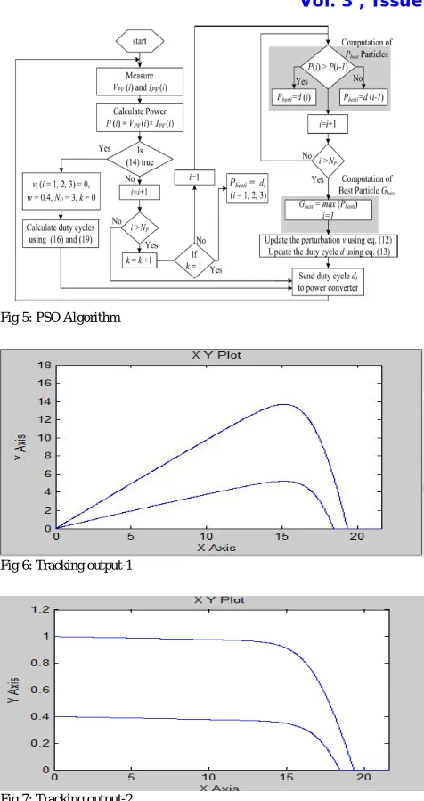
To obtain the maximum power from the PV modules, MPPT is normally employed. Over the years, various MPPT methods are proposed; for example, P&O, IC, HC, NN, and FLC [4], [9], [12], [15]–[19], [22]. In particular, the conventional HC method is interesting as the duty cycle of the power converter can be varied directly [16]. This can be explained with the help of a flowchart asshowninFig.
3.Thealgorithmperiodically updates thedutycycle d(k)byafixed stepsize Φwiththedirectionofin- creasing power. The perturbation direction is reversed if P(k) < P(k − 1), an
indication that the tracking is not moving toward the MPP. This can be described by the following equation: dnew =dold
+Φ if P>Polddold −Φ if P<Pold. (10) A clear advantage of
Vol. 3 , Issue 4 , April 2014
IV. PSO-BASED MPPT
A. General Overview of PSO
PSO is a stochastic, population-based EA search method, modelled after the behaviour of bird flocks [30]. The PSO
algo- rithm maintains a swarm of individuals (called particles), where each particle represents a candidate solution. Particles follow a simple behaviour: emulate the success of neighbouring particles and its own achieved successes. The position of a particle is, therefore, influenced by the best
particle in a neighbourhood Pbest as well as the best solution found by all the particles in the entire population Gbest. The particle position xi is adjusted
xk+1 i = xk i +Φ k+1 i (11)
where the velocity component Φi represents the step size.
The velocity is calculated by
Φk+1 i = wΦk i + c1r1Pbesti −xk i+ c2r2Gbest−xk i (12)
where w is the inertia weight, c1 and c2 are the acceleration coefficients, r1, r2 ∈U(0, 1), Pbesti is the personal best position of particle i, and Gbest is the best position of the particles in the entire population. Fig. 4 shows the typical movement of particles in the optimization process. If position is defined as the actual duty cycle while velocity shows the perturbation in the present duty cycle, then (11) can be rewritten as
dk+1 i = dk i +Φ k+1 i . (13)
From (10) and (13), it can be seen that both HC and PSO algorithms have an equivalent structure. However, for the case of PSO, resulting perturbation in the present duty cycle depends on Pbesti and Gbest. If the present duty cycle is far from these two duty cycles, the resulting change in the duty cycle will also be large, and vice versa. Therefore, PSO can be thought of as an adaptive form of HC. In the latter, the perturbation in the duty cycle is always fixed but in PSO it
varies according to the position of the particles. With proper choice of control parameters, a suitable MPPT controller using PSO can be easily designed.
B. Application of PSO for MPPT
To illustrate the application of the PSO algorithm in
tracking
theMPPusingthedirectcontroltechnique,firstasolutionvector
of duty cycles with Np particles is determined, i.e. xk i = dg =[ d1,d2,d3,...,d j]
j =1 ,2,3,...,Np. (14)
The objective function is defined as
P(dk i ) >P(dk−1 i ). (15) To start the optimization process, the algorithm transmits three duty cycles di (i = 1, 2, 3) to the power converter. In Fig. 5, duty cycles d1, d2, and d3 are marked with triangular, circular, and square points, respectively. These duty cycles served as the Pbesti in the first iteration. Among these, d2 is
the Gbest that gives the best fitness value (which is the array
power), as illustrated by Fig. 5(a). In the second iteration, the resulting velocity is only due to the Gbest term. The (Pbesti
−d (i)) factor in (12) is zero. Furthermore, the velocity of
Gbest particle (d2) is zero due to the (Gbest−d (2)) factor in
(12) is zero. This results in a zero velocity and accordingly the duty cycle is unchanged. As a result, this particle will not contribute in the exploration process. To avoid such situation, a small perturbation in duty cycle is allowed, as shown in Fig. 5(b), to ensure the change in fitness value. Fig. 5(c) shows the particles movement in the third iteration. Due to the fact that all the duty cycles in the previous iteration attain a better
fitness value, the velocity direction of these particles remains
unchanged and subsequently they move toward Gbest along the same direction. In the third iteration, all duty cycles (di, i = 1, 2, 3) arrive at MPP with a low value of velocity. In the subsequent iteration, due to very low velocity, the value of the duty cycle is approaching a constant. Therefore, theoperatingpointwillbemaintainedandtheoscillationaround the MPP diminishes.
V.SOLAR MODEL IN MATLAB
A. Model of Solar Cell
The solar cell block from SIMSCAPE tool and is represented as a single solar cell as a resistance Rs that is
connected in series with a parallel combination of the following elements:
Current source
Two exponential diodes
Vol. 3 , Issue 4 , April 2014
The mathematical model of the PV cells is implemented in the form of a current source controlled by voltage, sensible to two input parameters, that is temperature (ºC) and solar irradiation power (W/m2). An equivalent simplified electric circuit of a photovoltaic cell is presented
in
Fig 1: Equivalent Circuit of Solar Cell.
The output current Iis given by equation (14), I = Iph - Is*(e
(V+IRs)/(N*Vs) - 1)
- Is2*(e
(V+I*Rs)/(N2*Vt))
-1)-(V+I*Rs)/Rp
(14)
Fig 2: Solar Array Model in MATLAB
The above figure 2 is the MATLAB model of solar array which has 72 solar cells connected in series to form a solar array. This model is developed with the help of Sims cape tool block. The solar cell in Simscape tool is developed using the equation 1. The solar array is connected to the resistive load to view its performance.
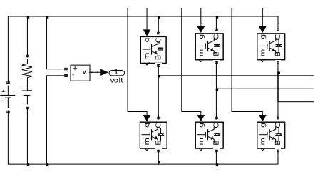
B. Model of Voltage Source Converter
Fig 3 MATLAB Implementation
Figure 3 shows the voltage source converter model consisting of six IGBTS. This voltage source converter is operated as the inverter for Solar farms during day time. During night time it is idle in condition as no power is generated hence it can be used for recative power compensation.
C. Simulation Results 1. General
The models are developed in MATLAB simulink environment. MATLAB (matrix laboratory) is a numerical computing environment and fourth-generation programming language. Developed by MathWorks, MATLAB allows matrix manipulations, plotting of functions and data, implementation of algorithms, creation of user interfaces, and interfacing with programs written in other languages, including C, C++, Java, and Fortran.
Fig4:PV Array -Simulation diagram
P
S +
-Variable Resistor I rradianc e
Vpv
Ppv
Ipv
+
-Soalr cell
Vary ing R Rvar P V
1000 Irradiance
I V
1 volt v +
-g
m
C
E
g
m
C
E
g
m
C
E
g
m
C
E
g
m
C
E
g
m
C
Vol. 3 , Issue 4 , April 2014
Fig 5: PSO Algorithm
Fig 6: Tracking output-1
Fig 7: Tracking output-2
Fig 8: PV system simulation
An additional package, Simulink, adds graphical multi-domain simulation and Model-Based Design for dynamic and embedded systems. MATLAB users come from various backgrounds of engineering, science, and economics. MATLAB is widely used in academic and research institutions as well as industrial enterprises.
Vol. 3 , Issue 4 , April 2014
2. Output Waveforms
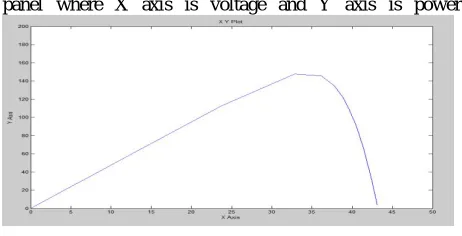
Fig 9 Voltage vs Power curve of Solar Cell
The figure 5.1 shows the voltage vs power curve of solar panel where X axis is voltage and Y axis is power.
Fig 10 Voltage vs Current curve of Solar Sell
The figure 5.2 shows the voltage vs current curve of solar panel where X axis is voltage and Y axis is current.
VI.PROPOSED MULTIPHASE DC–DC CONVERTER
A. Generalized Multiphase DC–DC Converter
BHB cell that is used as a building block of the proposed multiphase converter. Fig. 2 shows the generalized circuit of the proposed multiphase dc–dc converter for high- voltage and high-power applications. The generalized converter has “N” groups of converters, where each group of switch legs is connected in parallel at the low-voltage high-current side, while each group of voltage doublers is connected in series at
the high-voltage low-current side, i.e., “N” is the number of voltage doublers connected .
B. Operating Principles
The key waveforms of the generalized multiphase dc–dc con- verter are shown in Fig. 5. The interleaved asymmetrical PWM switching is applied to the multiphase converter, i.e., D and 1–D are the duty cycles of lower and upper switches of a leg, respectively, and each leg is
interleaved with a phase difference of 2π/(N·P). The average
value of the inductor current can be obtained.
Using (5)–(8), the ZVS currents and ZVS ranges of lower and upper switches as the function of input voltage and output power are plotted, respectively, as shown in Fig. 6. As shown in Fig. 6(a), the ZVS current of the lower switch tends to increase as the output power increases and decrease as the input voltage increases. This means that the ZVS turn-ON of the lower switch can be more easily achieved under the condition of higher out- put power and lower input voltage. It is noted that the ZVS range of the lower switch becomes broader for smaller total output capacitance Cos,tot = Coss,SL + Coss,SU of MOSFETs. For example, if MOSFETs with total output capacitance Cos,tot of 1.5 nF are selected in this example, the ZVS turn-ON of the lower switch can be achieved with output power, which is greater than 1000 W at input voltage of 40 V.
C. Interleaving Effect
Each leg of the multiphase converter is switched with a
phase difference of 2π/(N·P). The ripple frequency of the
input and input capacitor currents becomes N·P times the switching fre- quency of the main switch. The rms current of the input and input capacitor also decrease as N and P increases. The ripple frequency of the output capacitor current becomes P times the switching frequency of the main switch. The rms current of the output capacitor decreases as P increases. Due to the interleaved operation, the weight and volume of input capacitors,outputcapacitor,andinputinductorsaresignificantly
Vol. 3 , Issue 4 , April 2014
7 as a function of input volt- age and N. It tends to decrease as N increases in general.
A dc voltage is given as input, which is converted in to ac by controlled switches, which act as inverter when switches are off. Its output is given to the transformer, then to the voltage doublers, which rises the voltage level and the diode rectifier converter ac to dc voltage. Three phase inverter is connected for ac. load.
D . Interleaving Effect
The ripple frequency of the input and input capacitor currents becomes N•P times the switching frequency of the main switch. The rms current of the input and input capacitor also decrease as N and P increases. The ripple frequency of the output capacitor current becomes P times the switching frequency of the main switch. The rms current of the output capacitor decreases as P increases. Due to the interleaved operation, the weight and volume of input capacitors, output capacitor, and input inductors are significantly reduce.
The interleaving effect on the input capacitors CIU and CIL differs from that of the input inductor and output capacitor. The capacitor rms currents are calculated and as a function of input voltage.
E .Voltage Conversion Ratio
The ideal voltage conversion ratio of the proposed converter can be obtained by
VO/VS=N/(1–D)(NS/NP) (15)
Basically, as level of switches & diodes increases the voltage conversion ratio linearly increases. Considering the effect of voltage drop across the leakage inductance of the transformer, the actual voltage conversion ratio can be obtained .The actual voltage conversion ratio is plotted as a function of duty ratio D with different N and P,N is the number of switches and P is the number of diodes. It can be seen that as P increases the voltage conversion ratio also slightly increases (theoretically, it converges to the ideal voltage conversion ratio as P increases to infinity), since the effect of the voltage drop across the leakage inductance on the voltage conversion ratio becomes smaller.
VII. OPERATING PRINCIPLES
During positive supply voltage current flow through respective inductors, and upper switches ,and it
charges the upper input capacitors. When it charges to maximum voltage, it discharges and inductor transfer thecurrent to one side of corresponding transformer. Then corresponding upperswitches are open & negative supply voltage is given to the lower capacitor by corresponding lower switches and it is also available for the transformer and in this way the transformer get both the positive and negative voltage. The output of the transformer given to the voltage doubler and its DC output converted into AC by a three phase inverter. Its output used for running IM.
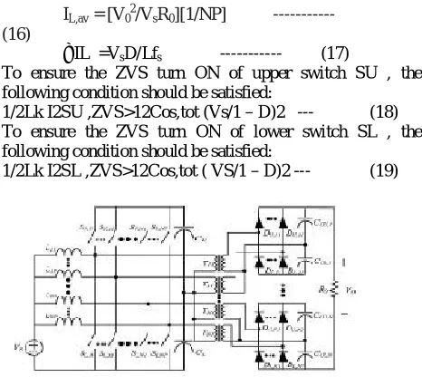
The average value of the inductor current is:
IL,av = [V02/VsR0][1/NP] --- (16)
∆IL =VsD/Lfs --- (17)
To ensure the ZVS turn ON of upper switch SU , the following condition should be satisfied:
1/2Lk I2SU ,ZVS>12Cos,tot (Vs/1 – D)2 --- (18) To ensure the ZVS turn ON of lower switch SL , the following condition should be satisfied:
1/2Lk I2SL ,ZVS>12Cos,tot ( VS/1 – D)2 --- (19)
Fig. 11. Proposed multiphase dc–dc converter (N is the number of series-Connected voltage doublers, and P is the number of diode legs connected to thesame output capacitors).
Vol. 3 , Issue 4 , April 2014
VIII.SIMULATION RESULT
A.Simulation Diagram Of Proposed System
Fig 12 Simulation diagram of proposed system
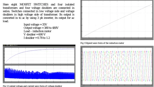
Here eight MOSFET SWITCHES and four isolated transformers and four voltage doublers are connected in series. Switches connected in low voltage side and voltage doublers in high voltage side of transformer. Its output is converted in to ac by using 3 ph inverter, its output for ac load.
Input voltage = 35V Output voltage = 380 to 480V Load – induction motor V doubler = 600 V I doubler = 0.78 to 1.2
Fig 13 output voltage and current wave form of voltage doubler
Fig 14 AC input voltage and output current wave form for the IM with filter
Fig 15Speed wave form of the induction motor
Vol. 3 , Issue 4 , April 2014
IV.CONCLUSION
The conventional system can only be used for DC load application and not for AC load also the voltage and current rating of the devices in the system are high. These drawbacks are overcome in proposed system by using 3 phase inverter and thus it can be applied fro ac load. The current and voltage rating of the devices are reduced by increasing the number of switches and diodes which also increases the output voltage. In future the output voltage can be increased further by increasing the number of switches and diodes.
REFERENCES
[1] A. R. Prasad, P. D. Ziogas, and S. Manias, “Analysis and design of a three-hase offline DC–DC converter with high-frequency isolation,” IEEE Trans. Ind. Appl., vol. 28, no. 4, pp. 824–832, Jul./Aug. 1992. [2] D. de Souza Oliveira, Jr. and I. Barbi, “A three-phase ZVS PWM
DC/DCconverter with asymmetrical duty cycle for high power applications,” IEEE Trans. Power Electron., vol. 20, no. 2, pp. 370–377, Mar. 2005.
[3] D. S. Oliveira, Jr. and I. Barbi, “A three-phase ZVS PWM DC/DC converter with asymmetrical duty cycle associated with a three-phase version of the hybridge rectifier,” IEEE Trans. Power Electron., vol. 20, no. 2, pp. 354–360, Mar. 2005.
[4] H. Kim, C. Yoon, and S. Choi, “A three-phase zero-voltage and zero- current switching DC–DC converter for fuel cell applications,” IEEE Trans. Power Electron., vol. 25, no. 2, pp. 391–398, Feb. 2010. [5] J. Lai, “A high-performance V6 converter for fuel cell power
conditioning system,” in Proc. IEEE VPPC 2005, pp. 624–630. [6] R. L. Andersen and I. Barbi, “A three-phase current-fed push–pull DC–
DC converter,” IEEE Trans. Power Electron., vol. 24, no. 2, pp. 358– 368, Feb. 2009.
[7] S. Lee and S. Choi, “A three-phase current-fed push-pull DC-DC converter with active clamp for fuel cell applications,” in Proc. APEC 2010, pp. 1934–1941.
[8] H. Cha, J. Choi, and P. Enjeti, “A three-phase current-fed DC/DC converter with active clamp for low-DC renewable energy sources,” IEEE Trans.Power Electron., vol. 23, no. 6, pp. 2784–2793, Nov. 2008. [9] S. V. G. Oliveira and I. Barbi, “A three-phase step-up DC-DC converter
with a three-phase high frequency transformer,” in Proc. IEEE ISIE 2005, pp. 571–576.