LinkIt: design, development and testing of a semi-quantitative computer modelling tool.

(1)

LinkIt: Design, development and testing of a

semi-quantitative computer modelling tool

by

FABIO FERRENTINI SAMPAIO

Thesis submitted in part fulfilment of the requirements of the Ph.D. degree

Department of Science and Technology Institute of Education,

University of London.

(2)

ABSTRACT

This research is about the design, development and testing of a semi-quantitative computer modelling tool called Linklt.

The aim of the software is to provide secondary students with a computational environment where they can think at a system level about models and the modelling process by expressing and testing their own ideas about phenomena without having to pay attention to the analytical relations between the variables involved.

The research involved two exploratory studies using two different versions of the software. These studies were carried out in Rio de Janeiro - Brazil with students aged 13-18 years old. During the studies, the students worked in pairs and used the computer tool to perform the expressive and exploratory tasks presented to them. The interviews were tape-recorded, some were also video-recorded and the models used and created by the students together with the steps to create them were saved and used for later analysis.

The design of the first version of the software - Linklt I - was based on an analysis of another computer modelling system called IQON. This first version of the software was then tested with students during a Preliminary study.

The analysis of the data collected led to a rethinking of the conceptual model of the system. A new interface and changes in the properties of the objects of the system were discussed and implemented, resulting in a new version of the software: Linklt II .

(3)

ACKNOWLEDGEMENTS

I am finishing this work with a strong belief that working with models can help us a lot to understand the world around us. However, in some circumstances, interacting with the "real thing" is a much better approach. During these last 4 years doing my PhD. at the Institute of Education I had the opportunity to work with Professor Jon Ogborn who is, with no doubt, a "real" supervisor (and not just a model of a supervisor). Among other important characteristics, he is a person who gathers all the necessary conditions to introduce students into the research realm and to make them think deeply about it. During this time he has been continually available to me, offering advice, suggestion and encouragement. For all of this I am deeply grateful to him.

We cannot pretend do a PhD. without undergoing a deep reflection of our "life beyond the PhD.". Doing a PhD. influences a lot the way we live and how we live influences a lot our PhD. as well. This process can well be seen as a feedback loop - although of high complexity ! - which over time alternates between positive and negative cycles of dominance. To take me out of many self reinforcing cycles that could have led me nowhere and put me back in a more well balanced feedback cycle I had to count on at least four special friends I made here in London: Isabel Martins & Joel Castro, Fani Stylianidou and Laercio Ferracioli.

May I also thank my partner Rita de Cassia. Her love, care and support has been invaluable, making me happier and more confident in my work.

There are other people that also became important persons for me: Paulo Adeodato and Sandra Leistner who shared a house and feelings with me for two years here in London; Carlos Perez, Ligia Barros and Arion Kurtz dos Santos which whom I exchanged thousands of emails where they were always supportive and informative.

I would like to thank all my colleagues who shared the research room with me as well as the staff of the Science and Technology Department. A special thank goes to Angela Kight and Janet Maxwell at the Technicians room.

I am grateful to all my colleagues of the Nude° de Computacao Eletronica at Universidade Federal do Rio de Janeiro - Brazil, for permitting my absence over the last four years and also to CNPq for its financial support.

In addition I would like to thank the schools that helped me to carry out my field work: Colegio de Aplicacao da U.F.R.J., Centro Educacional de NiterOi, Colegio Sao Paulo and Escola Tenente Antonio Joao.

(4)

LIST OF APPENDICES

APPENDIX A: PRELIMINARY STUDY: Support Texts Given to

the Students 296

APPENDIX B: CORE STUDY: Worksheets and Support Texts

Given to the Students 301

APPENDIX C: PRELIMINARY STUDY: Sample of a Case Study 309

(12)

LIST OF TABLES

Chapter 5

Table 5.1: Description of the groups and number of meetings

needed 113

Chapter 6

Table 6.1: A summary of dynamic modelling possibilities of

Linklt II 137

Table 6.2: Values of the variables involved in a simulation of the model about pollution shown in Figure 6.23. The first column of

pollution of the air corresponds to the value of its amount level.

The second column corresponds to its trigger level 155

Table 6.3: Values of the variables involved in a simulation of the

model about predator-prey shown in Figure 6.25 162

Chapter 7

Table 7.1: Summary of the tasks proposed 169

Table 7.2: Description of the groups, total number of meetings and meetings missed by one of the components of a certain

group 169

Chapter 10

Table 10.1: Group H working with the model about pollution in

big cities (Task 8) 256

Table 10.2: Group A working with the model about migration to

big cities (Task 4) 258

Table 10.3: Group E working with the model about diet and

healthy life (Task 6) 260

Table 10.4: Group C working with the model about diet and

(13)

LIST OF FIGURES

Chapter 2

Figure 2.1: A piece of program using DYNAMO language used

to generate the graph shown in Figure 2.2 35

Figure 2.2: An output plot produced by DYNAMO 35

Figure 2.3: The general architecture of DMS 36

Figure 2.4: DMS screen showing a graph of a model (growing

function) and the corresponding equations (right side) 37

Figure 2.5: Macintosh system interface 38

Figure 2.6: (a) Causal loop diagram with three variables (b) Causal loop diagram with three variables including a feedback

loop 40

Figure 2.7: Causal loop diagrams containing feedback loops:

(a) Positive feedback loop (b) Negative feedback loop 41

Figure 2.8: STELLA: Model about inflow/outflow of a tank with

its set of equations 43

Figure 2.9: Defining the mathematical computation of a variable

in STELLA 45

Figure 2.10: The underlying model is not consistent with the

visual presentation 47

Figure 2.11: IQON screen with a simple model about Population 48

Figure 2.12: A causal diagram corresponding to the model

shown in Figure 2.11 49

Figure 2.13: Graph of the variable Population X Time for the

model shown in Figure 2.11 51

Figure 2.14: Correspondence between an IQON model, Causal

(14)

Figure 2.15: Main window of ScienceWorks Modeler showing a digitized image of a river and two factors (Midge Fly:count and

Stream:oxygen) related to this problem 57

Figure 2.16: Object editor window showing the factors of the objectstream. According to this window the factor oxygen is affected by the factor MidgeFly:count and affects the factor

Stream:quality 58

Figure 2.17: Relationship Maker window. Specifies the type of relationship between factors. Here the factor Mayfly:count

affects the factor Stream:oxigen by increasing it in a linear way 58

Figure 2.18: Factor Factory window. Used to define the range of

variation and initial values of a certain factor 59

Chapter 4

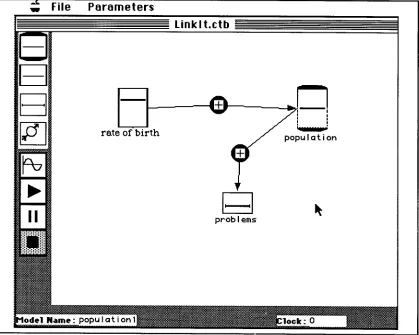
Figure 4.1: A simple model with Linklt: The screen objects rate

of birth, population and problems are known as Linklt's

variables. The arrows between them are known as links 73

Figure 4.2: How the computer screen looks like when Linklt is

loaded 75

Figure 4.3: Linklt's window with a model being constructed. The button related to the creation of links is selected on the Control panel. The appearance of the cursor on the screen resembles the operation in progress (create a link). If the user wants to create a link between level of alarm and industries-smoke, he/she has to click first on the variable box level of alarm (the system will highlight it to show that it was selected) and

afterwards on the variable industries-smoke 76

Figure 4.4: Control Panel 77

Figure 4.5: (a) An 'immediate' variable 'bigger than zero' (b) An 'immediate' variable 'smaller than zero' (c) A 'gradual' variable

'bigger than zero' (d) A 'gradual' variable 'smaller than zero' 80

(15)

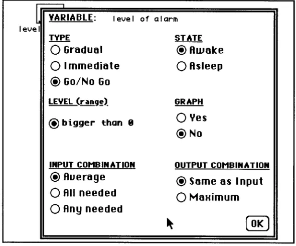
Figure 4.7: Information Box of an 'immediate' Variable 82

Figure 4.8: Information Box of a `GONOGO' Variable 82

Figure 4.9: Links: Types and Strengths 83

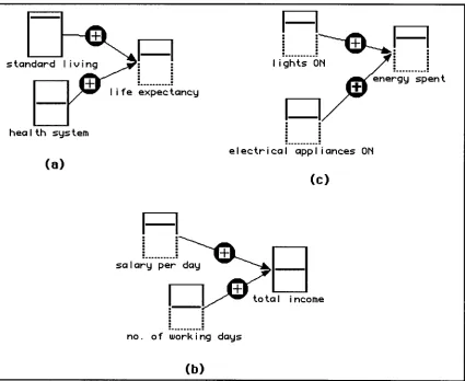
Figure 4.10: Three examples of algebraic models: (a) Model about life expectancy using 'average' combination; (b) Model to calculate the total income of a worker based on the salary paid per day and the number of working days in a month (use of `need all' as an approximation to multiplication); and. (c) Model to calculate the energy spent by the light bulbs and the

electrical appliances that are ON (use of 'need any' as an

approximation to addition) 84

Figure 4.11: Linear Processes - Graphical solutions 85

Figure 4.12: Examples of a linear process modelled with Linklt I 86

Figure 4.13: Exponential growth/decay - graphical solutions 86

Figure 4.14: Examples of exponential growth and decay

modelled with Linklt I 87

Figure 4.15: Model about Population - Combining exponential

growth and decay 87

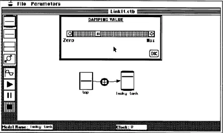
Figure 4.16: Example of an exponential decay model using the

`damping value' 88

Figure 4.17: Example of a second order derivative model 88

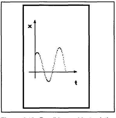
Figure 4.18: Example of oscillation with Linklt I 89

Figure 4.19: Possible graphical solution for oscillation-type

problems 89

(16)

Figure 4.21: An example of a simple model about population

before running ₉₉

Figure 4.22: The same model about population after 88

iterations ₁₀₂

Chapter 5

Figure 5.1: Model about water-cycle presented to the students 111

Figure 5.2: Group D: Model about money with a feedback loop 122

Chapter 6

Figure 6.1: (a) Smooth Variable (positive values) (b) Smooth Variable(any value) (c) On/Off Variable (positive values,

triggered) (d) On/Off Variable (any value, not triggered) 130

Figure 6.2: Information Box of a Smooth Variable 131

Figure 6.3: Information Box of an On/Off Variable 131

Figure 6.4: Different strengths and directions of cause of `go together' Links: (a) same direction/ normal strength; (b) same direction/strong strength; (c) same direction/weak strength; (d) opposite direction/normal strength; (e)opposite direction/strong

strength; (f) opposite direction/weak strength ₁₃₃

Figure 6.5: Different strengths and directions of cause of

cumulative Links: (a) same direction/ normal strength; (b) same direction/strong strength; (c) same direction/weak strength ; (d) opposite direction/ normal strength; (e)opposite

direction/strong strength; (f)opposite direction/weak strength 133

Figure 6.6: Information Box of a `go together' Link ₁₃₄

(17)

Figure 6.8: Two examples of algebraic models: (a) A model about the total income of a waiter where deductions is being subtracted from tips and salary (b) A model about clouds and sun shining. How much of sun shining is the inverse of clouds

in the sky (combining 'multiplication' and 'opposite' link) 136

Figure 6.9: Three different values (and interpretations) for the output of an 'On/Off' variable. In the first case the output is set to `high', in the second case it is set to low' and in the third case it

is set to 'equal to' 136

Figure 6.10: Two examples of linear process ( (a) and (b)) and its general representation with LinkIt II (c). The different signs of the links (in (c)) determine the value of the constatnt K in the

equations 138

Figure 6.11: Build-up exponential process: An example of a simple model about eye-pupil. The values of the variables are the initial conditions before the simulation. The variable pupil

size started with a value smaller than normal light level 139

Figure 6.12: Build-up exponential process: An example of a simple model about eye-pupil. The values of the variables are the initial conditions before the simulation. The variable pupil

size started with a value bigger than normal light level 140

Figure 6.13: General structure of an exponential process with Linklt II. The different signs of the links determine the value of

the constant K in the equations 140

Figure 6.14: An incomplete model about body growth producing

an exponential growth 141

Figure 6.15: Example of a population model. In this case exponential decay can be achieved by setting the variable

births 'asleep' 141

Figure 6.16: Exponential decay/growth can also be achieved using the 'changes by itself' parameter. Case (a) has this

(18)

Figure 6.17: Example of an Harmonic oscillator 143

Figure 6.18: Linklt's window with a model being constructed 144

Figure 6.19: Control Panel 145

Figure 6.20: Dialogue box to set the speed of simulations 148

Figure 6.21: Graph of Linear_Value (x) = Logn((1+x)/(1-x)) 149

Figure 6.22: Activation function with output equal to the amount

level 149

Figure 6.23: Activation function with output maximum 150

Figure 6.24: Activation function with output minimum 150

Figure 6.25: Model about pollution. The variables are set by the

user before a simulation 153

Figure 6.26: Model about pollution after 52 iterations 157

Figure 6.27: Model about predator-prey before simulation 158

Figure 6.28: 'Changes by itself' values set to rabbits and foxes 159

Figure 6.29: Model about predator-prey after 132 iterations 162

Chapter 8

Figure 8.1: Model presented to the students as an example of

what can be done with the software 173

Figure 8.2: Second model presented to the students as an

example of what can be done with the software 173

Figure 8.3: Model MEstra 177

Figure 8.4: Model about parking place (to be completed with the

(19)

Figure 8.5: Model using an 'On/Off' variable to introduce the

idea of 'triggering when below' 182

Figure 8.6: Model about predator-prey 183

Figure 8.7: Correct model about eye-pupil presented to the

students 184

Figure 8.8: Model about eye-pupil with two links changed.

Groups E and B used this model 184

Figure 8.9: Model about a refrigerator working 186

Chapter 9

Figure 9.1: Group E: A model about a punctured ball 191

Figure 9.2: Group C: Model about migration to big cities:

Exodus seems to be an independent variable 193

Figure 9.3: Typical use of 'On/Off' variable (model about

migration to big cities) 194

Figure 9.4: Group E: Model about a heating system: Heater turns on when above the threshold. Indoor temp. turns on when

below the threshold 195

Figure 9.5: Group C: Model about eye-pupil - Using a

"modelling gadget" to represent the idea of passing through a tunnel (the variable Tunnel is triggered when it is above the

threshold) 196

Figure 9.6: Group D: Model about pollution using "modelling gadgets" to implement a constraint on the variable use of cars

and use of public transport 197

Figure 9.7: Group E: Model about predator-prey: Using an 'any

(20)

Figure 9.8: Group H: A model about parking place using an `any value' variable to represent different moments of a certain

situation 202

Figure 9.9: Group E: Model about diet and healthy life. Making

variables `asleep' to try out an idea 205

Figure 9.10: Group I: Last model about diet and healthy life.

The variable age is set to increase 206

Figure 9.11: Group E: Model about money and shopping 212

Figure 9.12: Model suggested by Fabricio using 'cumulative'

links 216

Figure 9.13: Group H: Model about diet and healthy Life. For the students the variable diet should begin with an initial value to

represent the idea of someone beginning with a "good diet" 217

Figure 9.14: Group H: First model about pollution 224

Figure 9.15: Group J: Model about pollution. Seeing the

relations as 'inverse' 227

Chapter 10

Figure 10.1: First model about health and good diet (Group D): The model was mainly to 'calculate' how good or bad is

someone's health 233

Figure 10.2: Last model about health and good diet (Group D): The model was mainly to show someone's health evolving

during time passing 234

Figure 10.3: Model about diet and health used by the students

to discuss about their own health (Group J) 235

Figure 10.4: Model about eye-pupil presented to Group E 236

(21)

Figure 10.6: Group J: First version of the model about migration

to big cities 244

Figure 10.7: Group J: Last version of the model about migration

to big cities 245

Figure 10.8: First model about the heater (Group J) 247

Figure 10.9: Group J: Intermediary version about the heater.

Outside temperature is representing cold temperatures only. Inside temperature can represent cold temperatures (above the

middle) and hot temperatures (below the middle) 248

Figure 10.10: Group J: Last version of the model about the

heater 248

Figure 10.11: Group J: Model about resistance to smoking 250

Figure 10.12: Group C: Model about pollution of the air 252

Figure 10.13: Group H: Last model about pollution: Three

variables representing different types of pollution 257

Figure 10.14: Group A: Model about migration to a big city.

Later jobs on offer became attractives 257

Figure 10.15: Group E: First model about diet and healthy life 259

Figure 10.16: Group E: Sophisticated model about diet and

healthy life 260

Figure 10.17: Group C: First model about health and diet 261

Figure 10.18: Group C: Mechanism created to implement the idea of health changing with time and different consumption of

meat and dairy products 263

Figure 10.19: Group D used a reason from the real world for

(22)

Chapter 11

Figure 11.1: Main research questions and design of the studies 275

Figure 11.2: Model about migration to big cities created by

Group C at the end of the first meeting 277

Figure 11.3: Model about a refrigerator working showed to the

students during an exploratory task 278

LIST OF CHARTS

Chapter 4

Chart 4.1: Interface Operations 91

Chapter 6

Chart 6.1: Objects and Their Properties 128

Chart 6.2: Interface operations 146

Chapter 10

Chart 10.1: The three steps followed by the students when

(23)

PART I

(24)

Chapter 1:

MODELS AND COMPUTATIONAL

MODELLING IN EDUCATION

1.1 INTRODUCTION TO THE THESIS

The use of information technologies in schools is as diverse as the different theories that support them. However, they have a common paradigm: Information technologies somehow have the potential to augment the cognitive faculties of the learners (Chen, 1994). The term "cognitive tool" is thus used to refer to tools that have some cognitive properties or tools that are usefully employed in the performance of cognitive tasks (Kozma, 1987; Nickerson, 1988).

This thesis is concerned with the second of these two possibilities. In particular, it is about the design, development and testing of a computer modelling system to help students to externalise their thoughts and to think about them.

(25)

1.2 THE APPROACH

This work consists of four main parts. The first part (Chapters 1 to 3) presents modelling systems, discusses some research using these systems in educational settings and discusses the rationale for the present research. The second part (Chapters 4 and 5) is about the design, implementation and Preliminary study of a first version of a modelling tool, Linklt (Prototype I). The third part (Chapters 6 to 10) considers, on the basis of the Preliminary study, the design and implementation of a second version of the software (Prototype II) and presents a Core study in which the tool was used. This gives an account of students' ability to manage the software and to express/ explore their knowledge in a number of domains. The fourth and last part (Chapter 11) summarises the findings of the research and presents some ideas for further research.

1.3 MODELS AND MODELLING SYSTEMS

A model is a new 'world' that someone constructs to represent things from our world or from an imaginary one. Generally such models are simpler than the world they represent and we can work (or interact) with them to understand how things function both in the model world and, perhaps, in the modelled world as well.

Another important aspect of models and the process of modelling is that the same reality can be modelled in different ways, representing different aspects of the problem or different views of the modeller. A model of the economy of a country and its implications for inflation can, for example, be very different from different political perspectives. But here what is most important is the possibility the model gives to discuss ideas about a certain problem.

The construction and use of models is not something restricted to scientific environments. Since the beginning of our lives we are accustomed to working with models. For example, when a child is asked to draw a house on a piece of paper, what she/he produces is a model of what she/he thinks is a house. Maybe the house is not very well scaled ( it could have windows bigger than doors, trees smaller than people) or not all the details are included, but the most important thing is that it represents some essential aspects of the child's point of view.

(26)

interested in a simplified system that simulates some significant characteristics of another system that, in this case, belongs to the real world. In its turn, a model of a bird (or a prototypical bird) is an ideal or standard one that can be used to make comparisons with or identify other animals.

Each of these examples captures a different aspect of modelling systems: they permit the representation of significant structures and events of a certain world; they have a set of rules that govern the functioning of their parts; and they can be used to compare/describe different representations (Sowa, 1984). Computer software that works in this way is called a computer-modelling system.

1.3.1 Simulations. Modelling and Computer Languages

At this stage it is important to differentiate modelling systems from other related applications like simulations and programming with computer languages.

A simulation is an attempt to imitate or approximate something imaginary or in the real world. If we are thinking about computer simulations we can see them as a piece of software that tries to mimic the behaviour of a certain domain. According to Steed (1992) the difference between models and simulations is that " (models are) a representation of structures whereas a

simulation infers a process of interaction between the structures of the model to create a behaviour ". In other words, simulations pay attention to the

results (output) given by the execution of the (hidden) model they contain.

In its essence a computer modelling tool is a computer language. What mainly differentiates one from the other is the level of granularity of their primitives. In conventional computer languages the primitives are more general (and elementary) - so as to permit the exploration of many fields - while requiring more programming skills of users to develop their own models. However, as the problems to be presented in modelling systems are more specific, the set of conceptual primitives existing in these systems can be more powerful (though less general), requiring less programming skills of its users.

A modelling system could be used to create both models and simulations. For instance, you could use a modelling system like STELLA (Steed, 1992) to create a model to represent the interrelations among the employees of an industrial company and permit people who are interested in increasing the profits of the company, to try some simulations with that model, changing some its parameters (e.g. salary of the employees).

(27)

is easy to construct, modify/adapt and test models about a certain domain under certain conditions.

1.4 MODELLING SYSTEMS: A CLASSIFICATION

There are many different characteristics of modelling systems that could be used to classify them. As this study is mainly concerned with models that can be implemented computationally and focuses on aspects related to their use in educational environments, I will use a classification devised by Bliss & Ogborn ( Vac) that focuses on the way to express the ideas to be modelled ( For more information see (Gilbert & Osborne, iiso ; Ogborn, 1993).

1.4.1 Quantitative Models

Quantitative models are strongly based on variables and mathematical relations between them to describe (or to model) a situation in the world. So to describe a situation, the user must be able to identify its variables and specify the exact functional relation between them. From this perspective, if someone wants to explain how the velocity of car is changing over a certain period of time, it would be necessary to have an equation system like this:

V:=V +a*DT X:=X+V*DT a := ?

DT := ? Vinitial := ? Xinitial := ?

(28)

environment, the concept of object orientation and four basic building blocks to implement a fluid flow analogy (Richmond, 1987) (see Chapter 2 for further description of STELLA).

Older systems exist and are still in use. They are normally programmed in BASIC (Kurtz dos Santos, 1995) and permit the user to either enter some parameters required by the simulation or to introduce a module that describes the event to be modelled. An example of this second case is the DMS system developed for BBC computers (Wong, 1986).

An interesting case is the increasing use of spreadsheets as quantitative modelling system by teachers. Brosnan in Mellar, Bliss, Boohan, Ogborn, & Tompsett (1994: 76-77) gives two reasons for this. First, worksheets give students the possibility to focus their attention on their understanding of the underlying scientific principles of a phenomenon, leaving to the software the (almost total) control of the "mechanical mathematics" that governs the phenomenon, and second, they can be used in many different conceptual areas across the curriculum.

1.4.2 Qualitative Models

Qualitative models are based on a descriptive specification of the objects and their relations in the world to be modelled. In our daily life we are familiar with this mechanism for explaining to someone else how things function. Although such qualitative models are not very suitable in applications where you want to repeat or simulate situations in an automatic way, some computational modelling systems like Linx88 (Briggs, Nichol, Brough, & Dean, 1989), VARILAB (Hartley, Byard, & Mallen, 1991) and 'Explore your Options' (Bliss & Ogborn, iqqia _{), permit such descriptions to be made using a graph}

metaphor, with nodes (objects) and links (relationship between objects), so that some automation can be achieved.

1.4.3 Semi-quantitative Models

(29)

It might be thought that this kind of construction is only used by naive or 'plain folks' to explain the behaviour of certain situations, but researchers in the artificial intelligence and cognitive science communities have argued that semi-quantitative reasoning also seems to be used by experts to express causal explanations of the behaviour of physical systems (de Kleer & Brown, 1983; Dillon, 1994; Kuipers, 1994). One possible consequence of this argument is that semiquantitative modelling systems can contribute to a deeper understanding about the world by permitting people to externalise and discuss their ideas about a certain domain, focusing on the conceptual level of the problem instead of its functional level.

1.4.4 Dynamic versus Static Models

Another important dimension of modelling systems is their relation with time. Modelling systems that permit the construction of models that change over time are called dynamic modelling systems. Otherwise they are static modelling systems . So a modelling system that permits the construction of dynamic models has to have one module that permits the modeller to express the concepts and ideas to be modelled (representation module) and another that is responsible for calculating the evolution of the model over time (processing module), giving feedback to the modeller. However, static modelling systems may not need a processing module. A good example is a hypertext system used to represent someone's ideas about the most interesting tourist places in London. Static modelling systems that do have a processing module are mainly concerned with the satisfaction of constraints. An example is a spreadsheet used to calculate the impact on the profit of a company if you raise the salary of its employees.

One important aspect of dynamic modelling systems is that they serve well to represent (and therefore to help to think about) real life situations. They are at the basis of the system dynamics framework (Forrester, 1968) which tries to understand certain phenomena by looking at them as a "collection of interacting elements that function together for some purpose" (Roberts, 1983) (see chapter 2 for a description of some computer modelling systems that use this approach).

1.5 COMPUTER MODELLING IN EDUCATION: WHY?

(30)

analysis of some common daily activities suggested and developed many artefacts that helped the execution of these activities, and postulated the first rules that led to the origin of mechanics. The objective of science is to understand and explain real-world phenomena. Models are at the heart of this activity as "thinking tools" to help scientists in their tasks.

To make students "science literate" is essentially to make them think in a critical way about scientific concepts and to question them (Papert, 1980; Steed, 1992; Wong, 1993). In such an educational setting the important thing is not only to make students find the correct answers but to give them the opportunity to become active learners, engaging in a process whereby they can develop their own understanding of natural phenomena. In such an educational environment computers can be used to,

...explore domains where the teachers know a bit more than the students, but do not know all the answers. Domains they could model with their class, around which they could cope with their students, about which they could share some healthful moment of discovery and amazement . (Vitale, 1988, p. 227).

The importance here therefore is not only to make students find the correct answer but to give them the opportunity to become active learners, engaging in a process where they can develop their own understanding of natural phenomena.

The best that can be done to understand the behaviour of the physical world is to guess intelligently some likely causes of that behaviour and construct mental representations of them. Following this individuals can formulate some hypothesis about the processes that are going on and predict some of their consequences. In some special circumstances, it is possible to go there (to the physical world) and test these hypotheses. These ideas of creating a model and some theories about them are, according to Gilbert & Osborne (1980: ,0), "the

`imaginative adventures of the mind' and they bring the essential ingredient of creativity into science".

Working with physical means of representation (e.g. pencil and paper) permits the externalisation of the concepts and meanings that are embodied in mental representations, helping the learner to think about what is intended to be represented (Novak & Gowin, 1984). Using a computer modelling system to represent concepts and meanings permits the learner to go further in his/her ideas, exploring the relations between the different kinds of objects, formulating and testing hypotheses, etc. About these ideas Webb (1990) suggests:

(31)

In order to assist children in improving their mental models so that they are closer to accepted scientific theory, it is necessary for teachers to provide a learning environment which will facilitate children in reconstructing their mental models. The conditions needed for this to occur are those in which the inadequacies of a child's mental model become apparent to that child and she/he can experiment with alternative models ... (p. 6-7)

Another important characteristic of computer modelling systems is the possibility of linking multiple representations which can facilitate the process of creating meaning from representations.

The issue of representation is crucial in science and science education. Science can even be defined as a means for constructing and improving representations of the world. (Teodoro, 1992b, p. 2).

1.5.1 Barriers to Accessibility

At the present time the main problem that persists with mathematical modelling systems is the "high entry fee" that has to be paid to use them. Some authors like O'Shea & Self (1987) argue that the physical sciences are very much concerned with the development and use of mathematical models, but that their complexities are, in most cases, beyond the students' abilities. This idea suggests that work with modelling should start from a more qualitative platform. When sufficient knowledge about modelling is developed and the mathematical skills are present, students could then migrate to modelling systems which offer more quantitative results (Ogborn, 1992). About this Kurtz dos Santos (1992) says:

...it is important to begin from a secure base in observed phenomena. Much of the empirical knowledge at this stage will be qualitative, in that quantitative formulations depend on later stages being achieved, such as variables being isolated and relationships postulated. This suggest an emphasis on simple experimental work aimed at a qualitative understanding of the system: what happens and what affects what happens. (p. 56)

(32)

a help system available), diverting his/her attention from the cognitive-relevant aspects of the problem. Also modelling environments that incorporate too many options and a large number of expert level modelling functions can easily discourage the new user.

1.6 MOTIVATION FOR PRESENT RESEARCH

Due to the constraints of mathematical models, some authors argue that the use of semi-quantitative modelling systems can be beneficial to people without a mathematical background, e.g. young students (Bliss & Ogborn, 1992). In considering the use of computers to implement semi-quantitative models an environment should be set up where the user is responsible for defining the variables and their relations and attaching to them some characteristics that reflect the functional aspects of the objects and events being modelled. The computer, in its turn, would be responsible for choosing the right equations to govern the evolution of the model from the characteristics of the variables and relationships already created by the user, and for making the model evolve over time.

In 1992 I became aware of research carried out by the London Mental Models Group (Bliss & Ogborn, 1992) which led to the development of a semi-quantitative modelling system called IQON (Miller & Ogborn, 1990) (see also Chapter 2). The research presented in this thesis builds on that research in the computer modelling field. A new semi-quantitative computer modelling tool - LinkIt - that is more general than IQON, but still simple to use, is proposed, designed, implemented and tested.

What follows in the next two chapters of Part I of the thesis is the presentation and discussion of some existing computer modelling systems that were influential for the design of the present system (Chapter 2) and the rationale for this research (Chapter 3).

(33)

Chapter 2:

RELATED WORK ON MODELLING

SYSTEMS

2.1 INTRODUCTION

This chapter presents the main ideas of the systems dynamic approach and describes and discusses three of the most important computer modelling systems developed within this approach. The chapter concludes by relating these computer environments to the software developed as part of this research.

(34)

2.2 SYSTEMS DYNAMIC APPROACH AND COMPUTER MODELLING FOR EDUCATION

Systems thinking - which is the concept behind the systems dynamic approach - grew rapidly at the end of the 1950s at MIT when Jay Forrester and some of his colleagues started using it to think about management problems. However the idea gained prominence in the 1960s when it was applied to urban growth and development and global patterns of the consumption of natural resources (Mandinach, 1989; Toval & Flores, 1987).

Systems thinking is a valuable tool for understanding the behaviour of complex systems over time using simpler concepts of change, causality and feedback. By specifying the rules that define the causal relationships between variables and how they change over time, it is possible to construct simple and general models that account for biological, ecological and societal problems.

In the last two decades, with the increasingly widespread use of microcomputers in schools, the systems dynamic approach has been used as the backbone of many of the computer modelling/simulation systems available for those computers (Millwood & Stevens, 1990). Most of these systems were written in BASIC and permit the students to manipulate some of their parameters. The outputs of these systems are either tables containing the values of the important variables against time or plotted graphics of these variables. Some examples of these systems can be found in Marx (1984) and Crandall (1984) who present a collection of simulation programs related to topics in mathematics, chemistry, physics and biology.

However, from an educational point of view, these computer programs have three major drawbacks: (i) they require time and computer skills for the users to enter the programs in the computer; (ii) they distract the user from engaging directly in the process of modelling; and (iii) they only permit the manipulation of some parameters, functioning more as a black box yielding little or no insight into the interrelationship of the elements of the system from which the output has arisen (Whitfield, 1988).

(35)

YEAST=Y, BUD DING=B

o.':•" ',a.,1(1 1 u tl.r.:) 1'0 . Cc. ;!:j _ a a o.0d6 ',.:1)) in . no; I.:. en': i ;I .:1:11; ,). C500 v ---.--- Y l

H TA . YU . rat re TH L _ ODD

• V t• 7 • fp Y6

r. _•

. Yli VH

. r

20 .Van

•

- -y -- D

• 113 Yid

• Y . VII

r Yb

Y yEl

. Yu Y • Ye - 3a.000 y Y B YEAST GROWTH

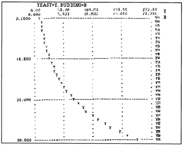
L YEAST.K = YEAST.J+(DT)(BUDDNG.JK)

N YEAST = 10

NOTE YEAST CELLS (CELLS)

R BUDDNG.KL = (YEAST.K) (BUDFR) NOTE BUDDING (CELLS/HOUR)

C BUDFR=0.10

NOTE BUDDING = FRACTION (1/HOUR) PLOT YEAST=Y/BUDDNG=B

PRINT YEAST,BUDDNG

SPEC DT=1/LENGTH=30/PLTPER=1/PRTPER=5 RUN

Figure 2.1: A piece of program using DYNAMO language used to

generate the graph shown in Figure 2.2

Figure 2.2: An output plot produced by DYNAMO

A second approach taken by other researchers is the development of computer dynamic modelling environments where the user just has to introduce a module that corresponds to the world to be modelled. Examples of this case are the systems MODL (Hartley, 1981), MECHANICS (Staudenmaier, 1982) and DMS (Dynamic Modelling System) (Ogborn & Wong, 1984; Wong, 1986).

(36)

integrating different but complementary tools in order to help the user to accomplish a certain task in a shorter period of time.

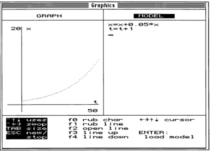
DMS can be seen as a good example of this category. It was initially developed in BASIC for BBC computers (versions for Mac and RML computers came later) and integrates, in the same environment, 3 modules that are essential for the modelling process: a program editor that permits the user to interact with the system (create models, load a previous one, change parameters, etc.); a graph plotter responsible for the output of the model when it is iterating; and an empty slot where the model (actually the equations that represent it) can be inserted (see Figure 2.3 and 2.4)

Program editor

Slot waiting for model

Graph Plotter

Figure 2.3: The general architecture of DMS

(37)

Graphics

GRAPH NuDEI_

20 x ... • • • t x=x+0.05'F'x t=t+1 50

1 4- -= -= = tO f1 f2 f3 f4

rub char .(-4.1.4. cursor

rub line open line

line up ENTER:

line down load model

-.I.. - t _■• . _..--1.._.

RE: f-:C

- ---ke.op si=e r-i.T-. .-.w./

t•=. •

Figure 2.4: DMS screen showing a graph of a model (growing function) and the

corresponding equations (right side)

A second negative aspect is that the outputs of these kinds of software are in the form of graphs and/or tables representing the values of the variables, which is not a straightforward way either to understand how the elements of the model are changing or to grasp a systemic view of the model evolving over time.

The idea of giving students full control to express and test their ideas about formal objects has become a common claim by many researchers working with computers in educational environments. However the computational metaphor of programming used so far was too basic to permit the exploration of certain fields. A new more powerful metaphor that gives students the possibility of concentrating on the objects and actions of the domain to be explored without having the burden of first having to program these domains was needed. The direct manipulation style of interface (Shneiderman, 1992) and causal loop diagrams (Roberts, 1983) provided new metaphors for a new family of computer modelling tools.

(38)

Menu bar Hard disc icon

Resizing Box Trash Icon

1=1 Macintosh HD

4 items 78.4 MB in disk 75.7 M3 availst

0

Special System Folder

ACESSCRIES Applications

/

0

IC> O

MEM

(Papert, 1980). The LOGO environment makes a great appeal of manipulating

computational objects, giving the student a sense of playing with a concrete

world. But rather like other computer-modelling software it needs to be

programmed.

2.3 DIRECT MANIPULATION INTERFACES

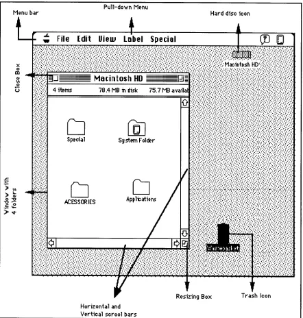
The most common example of a direct manipulation interface (also

referred to as a graphical object-oriented interface) is the Macintosh computer's

desktop. It contains icons (pictures) representing folders, documents, discs and a

wastebasket. It also contains windows which sometimes come with menu bars,

scroll bars and boxes for zooming, resizing and closing (see Figure 2.5).

Pull-down Menu

Horizontal and Vertical scrool bars

(39)

This style of interface is also known as a WIMP interface. The term "WIMP" is an acronym for Windows, Icons, Mouse and Pull-down (or Pop-up) menus which describe the main features of this type of interface.

An important concept in the realm of direct manipulation interfaces is that of metaphor. A metaphor can be seen as an "invisible web of terms and

associations that underlies the way we speak and think about a concept "

(Erickson, 1990, p. 66). Its purpose is to help in the understanding of abstract concepts starting from more familiar and understandable knowledgel.

The metaphor used by Macintosh computers is that of a desktop environment. The idea is to use the (hopefully) familiar concepts we already have about how the top of an office desk is organised to help to understand how to interact with the Macintosh system. Some familiar office objects are presented on the screen in the form of icons such as folders, files and a wastebasket. The user can "open" these objects to see and manipulate their contents.

However, it is important to notice that the desktop metaphor does not necessarily have to be the metaphor used by all graphical object-oriented systems. These two concepts have become so closely indentified in the computer interface world that people sometimes use them as synonyms. An example is the calculator existent in the same Macintosh environment mentioned above. When the calculator is evoked (normally by selecting it from the Apple menu) the system displays a drawing that resembles a pocket calculator. In order to use the computer calculator it is necessary to have knowledge of (in other words, to be familiar with) how a pocket calculator works. So, what is being used is familiar knowledge about how an electronic calculator operates, which is a different metaphor from that employed by the system.

The main advantage of direct manipulation interfaces is that their objects are dynamic and interactive. Instead of typing a line command such as "open a window and display the content of the hard disc on it", the user can directly double click on the hard disk to see its contents. So the user has a feeling that the displayed objects replace, or even become the objects and operations they represent (Clark,1993). Empirical studies have shown that after a very short period of use these objects can be manipulated without conscious attention (Smith, Irby, Kimball, & Verplank, 1982).

This style of interface is based on at least two assumptions that have important implications for the design of computer tools for education (Kozma, 1987):

• It gives the user the sense of manipulating concrete objects and therefore he/she can apply his/her knowledge of the world to interact with and understand them;

(40)

Cars +

Pollution of the air

(a)

Health

Industries

7

Amount of gasoline available

Price of gasoline Number of cars

on the road

(b)

• The actions upon these objects can be done in an "unconscious way", permitting a reduction in the cognitive load on the user and giving him/her the opportunity to concentrate on the work to be done. This is what Rutkowski (1982, p. 291) calls the principle of transparency: "The user is able to apply intellect

directly to the task; the tool itself seems to disappear".

2.4 CAUSAL LOOP DIAGRAMS

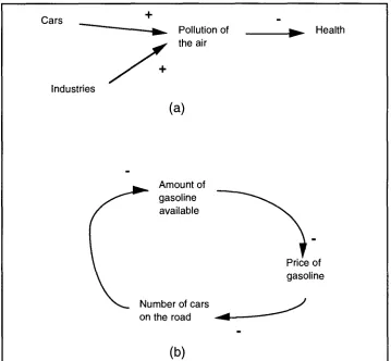
Causal loop diagrams are a graphical technique used to represent causal relationships between the elements of a problem being studied (see Figure 2.6).

Figure 2.6: (a) Causal loop diagram with three variables (b) Causal loop

diagram with three variables including a feedback loop

Basically they have three important elements:

• Nodes - Used to represent the elements (or variables) of the problem being

modelled;

• Arrows or links - Used to represent a causal relationship between variables.

(41)

(a)

+

Outside Temperature

Temperature of the room

Operation of the oil burner

(b)

amount of sale

+ Number of people Pm" in sales force

• Sign of the relationship - Indicates how a causal variable influences a

dependent variable. A positive influence means that as time changes, the variation of the dependent variable follows the same direction as the variation of its causal factor. In that way the example shown in Figure 2.6.(a) could be read like this: " If the number of cars increases the pollution of the air will increase". The complementary idea is also implied: " If the number of cars decreases the

pollution of the air will decrease".

A negative influence means exactly the contrary: the variation of the dependent variable goes in the contrary direction of the variation of its causal factor. In Figure 2.6.(b) the relationship between amount of gasoline available and price of gasoline could be read like this: " If the amount of gasoline available increases the price of gasoline will decrease. If the amount of gasoline available decreases the price of gasoline will increase ".

There are two other important concepts associated with causal loop diagrams: positive feedback loops and negative feedback loops. A positive feedback loop is when a causal loop diagram has a closed loop where the behavioural changes are reinforced. Over time, positive feedback loops have a tendency to present run-away growth or collapse as a consequence of the "snowball" effect (see Figure 2.7.(a)).

Negative feedback loops tend to reverse the direction of change as the loop is traversed. It is possible to see it as something resisting change or counteracting, over time, an external disturbance (see Figure 2.7.(b)).

Figure 2.7: Causal loop diagrams containing feedback loops: (a) Positive

(42)

The use of causal loop diagrams provides an easy way to introduce students and teachers to dynamic modelling for the following reasons (Roberts, 1983; Toval & Flores, 1987):

• It is a graphical representation based on very simple building blocks that permits more effective communication of someone's ideas about a system;

• It permits the visualisation of the whole model facilitating the "systems view" of the problem;

• It permits a sequential approach, by stages, for constructing models.

The three computer systems STELLA, IQON and ScienceWorks Modeler -described in the next sections are examples of how the ideas of direct manipulation interfaces and causal loop diagrams were put together to provide simple and yet powerful computer modelling tools for education.

2.5 STELLA SYSTEM

This section has two subsections. The first subsection gives a general description of STELLA (Structural Thinking Experimental Learning Laboratory with Animation) focusing on its building blocks and interface. This description is based on the writings of the following authors: Mandinach, 1989; Richmond, 1987; Steed, 1992; Whitfield, 1988.

The second subsection criticises the software assuming its use in an educational environment.

The STELLA version considered here is 2.01 for Macintoshes2. The system was tried both on a Power Macintosh 7100/80 and a Macintosh LC III.

2.5.1 STELLA: General Description

STELLA is a computer system designed for the representation of dynamic models using iconic levels, flows and converters. In a certain way it can be seen as an implementation of DYNAMO with a graphical interface.

The system takes the idea of causal loops and elaborates on them through a metaphor of tanks, pipes and flows, providing the user with four building blocks:

Stock - _{Represents a quantity that can increase (accumulate) or decrease} (de-accumulate) over time.

(43)

Flow _{- Controls the rate of incoming and outcoming material from} stocks. A Flow can come from or go to a 'cloud' which means that its source or destination are not specified (it can mean that the cause or effect of the flow is not relevant to the model). Flows can be altered by stocks and converters.

Converter _ Converts inputs into outputs. They can be constants or calculated from other quantities.

Connector - Connectors are used to determine that one variable in the model depends on one or more other variables in the same model.

Figure 2.8 below shows a model about inflow/outflow of a tank constructed with STELLA. There is also an inner window showing the (partially complete) mathematical equations that describe the model.

■f.

File Edit Windows Display Run

4

T

0 _{SC_______}

ig

r>

₄₁₁

level f_the_tank

inflow_rate outflow_rate h

o

--- gravity_constant velocity

. I.7.1 Equations _{III_}

• level_of_the_tank = level_of_the_tank + dt * ( inflow_rate - outflow_rate )

INIT(level_of_the_tank) = 100 0 gravity_constant = 9.8

0 inflow_rate = 20

0 outflow_rate = (statement goes here...) h

4 . _...

:.• •0, 0 velocity = (statement goes here...)

EA

(44)

The control panel on the left side of the window provides the elements to edit a model. The first four icons represent the four different building blocks provided in STELLA. To create a stock or converter, the user has to select one of these objects (single click) and point and click on the place he/she wants to place the object on the working area. The last three icons correspond to the tools to manipulate the building blocks: the fifth icon (the hand) is used to select and move items; the sixth icon (the ghost) duplicates an element that can be placed anywhere on the window; the last icon, the dynamite, serves to break existing connections and variables.

After drawing the model the user has to double click on the objects on the screen to set the equations and the initial conditions of the variables. After that it is necessary to set the scales (range of variation) for the objects created and run the model (both functions are inside the Run pull-down menu). Another way of relating variables of the system is through a graph (drawn by the user) that specifies the relation between two variables of the model.

The outputs of STELLA can be of 3 kinds:

- Animated diagram - The graphics capabilities of the system permit the user to see in real time the flow of information in the model. The levels of the stocks move up and down representing a tank being 'filled' or 'emptied'. Flows and converters have small arrows that move across their icons as a function of their value.

- Table - Show in a table the values of the objects chosen by the user.

- Graph pad - Show a graph of the objects chosen by the user. The system can show scatter plots of two variables or a time series graph of up to four different variables.

2.5.2 Mathematics of STELLA System

After creating a diagrammatic representation of a problem on the screen, the user has to describe how the elements presented on the diagram change in time and in respect to the values of other variables and constants.

(45)

Builtins AND FIRCTAN BEEP COS DELAY DT Required Inputs

0 velocity 4

'0,

outflow_rate = {statement goes here...)

Become Graph Cancel OK

O

0

)

outflow-rate. The system also provides a set of mathematical functions that can

be used by the user. They appear in the window called "Builtins".

Figure 2.9: Defining the mathematical computation of a variable in STELLA

After specifying the mathematical relations among the elements of the model the system can simulate it by solving the finite difference equations using one of three possible numerical methods (which can also be chosen by the user): Euler, 2nd-order Runge-Kutta and 4th-order Runge-Kutta .

2.5.3 Discussion of STELLA System

The most beneficial aspect of STELLA is its exploitation of a graphic interface to represent and animate the structural diagram of a given problem. With such a system it is possible for the learner to visualise changes to the whole system over time, permitting him/her to have a better understanding of phenomena.

Another positive aspect of STELLA is the different outputs it can present for a certain simulation. Discussing and linking the ideas embedded in these different outputs can help the process of creating meaning from different representations (Teodoro, 1994).

(46)

them by the user until he/she asks for the system to run the model. This can be cumbersome for the learner because he/she can not have a qualitative idea about the initial state of the model before starting a simulation.

The second problem is that although the system permits the user to set individual scales for the variables, it does not explicitly show these scales when the software is running. Again this can confuse the user specially in situations where he/she has many objects on the screen.

The third problem is about AkINNINC7 a model. Although the user can set

the number of iterations for a certain simulation, the system does not provide a way to control how fast it is going to run a simulation. So, if the user creates a model with just three or four variables it will be very difficult to visually keep track of the changes of the variables while the model is running. This becomes specially difficult using a fast machine.

The next three problems are more fundamental and have to do with how the system was conceptualised and with how the visual metaphor is used to represent models.

The system's conceptual model is based on a metaphor of values flowing in and/or out of stocks. To represent these two kinds of flow, the system uses an icon called flow which resembles an arrow indicating the direction of flow. So a flow starting on a stock and going to the clouds gives the expectation that the stock is being de-accumulated (an out-flow). A flow finishing on a stock (an in-flow) gives the expectation of a stock accumulating. However if the user gives negative values for the flows, they will behave in the contrary way: an in-flow with a negative value will make the stock empty. In the same way, an out-flow with a negative value will make the stock fill up. So what we have here is a compromise between the mathematics of the system and the way it is presented by the interface. If we recall that STELLA was developed for students being initiated into modelling, then the visual representation of a model must have much more importance than the mathematics that goes behind it. As a result, at least for beginners, the model presented in Figure 2.10 can have a certain inconsistency between what is shown on the screen and the results of its simulation (with

Mortality being negative, Population will increase instead of decreasing).

Another inconsistency between the mathematics and the visual metaphor of the system is that although it is possible to have negative values in the underlying model (at the mathematical level), the minimum visual value for a stock on the screen is zero ('empty').