Article
1
Machine learning for the design and development of
2
biofilm regulators
3
Benjamin Stone and Erik Sapper*
4
Department of Chemistry and Biochemistry, California Polytechnic State University, San Luis Obispo, CA
5
93407. *Corresponding author: [email protected]
6
7
Abstract: Biofilms are congregations of bacteria on a surface, and they grow into obstacles for the
8
functionalities of any device or machinery involves anything biological. Biofilms are developed
9
through a biochemical system known as ‘Quorum Sensing’ that accounts for the chemical signaling
10
that direct either biofilm formation or inhibition. Computational models that relate chemical and
11
structural features of compounds to their performance properties have been used to aide in the
12
discovery of active small molecules for many decades. These quantitative structure-activity
13
relationship (QSAR) models are also important for predicting the activity of molecules that can have
14
a range of effectiveness in biological systems. This study uses QSAR methodologies combined with
15
and different machine learning algorithms to predict and assess the performance of several different
16
compounds acting in Quorum Sensing. Through computational probing of the quorum sensing
17
molecular interaction, new design rules can be elucidated for countering biofilms.
18
19
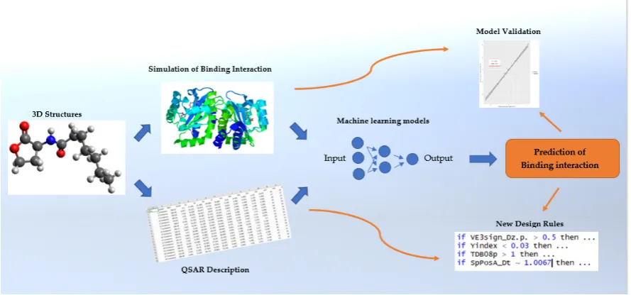
Figure 1. Graphical abstract of this study’s workflow
20
Keywords: Machine Learning: Biochemistry;QSAR; Molecules; Neural Networks
21
22
1. Introduction
23
Biofilms are a buildup of bacteria that form on a surface and disperse bacteria colonies. Bacterium
24
individually are known as ‘planktonic’ and exhibit individual locomotion, but once a certain
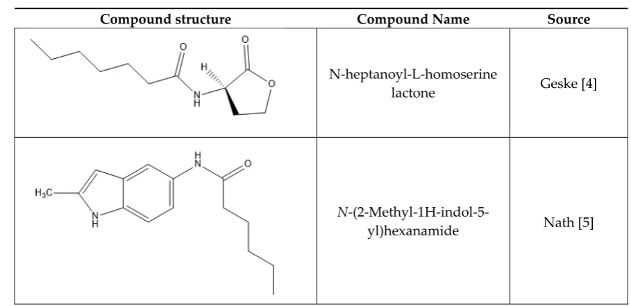
25
population (or quorum) congregates on a surface, specific intracellular signals are produced [1]. This
26
process is called ‘Quorum sensing’ (QS) and it consists of the chemical communications bacteria use
27
to either turn on or turn off the biofilm formation and growth response. Chemical signals or ‘quorum
28
sensors’ are part of the protein interactions causing the group of bacteria to switch their gene
29
.
expression to one that facilitates biofilm regulation. These chemical signals are called auto-inducers
30
[2]. Auto-inducers start the transcription process for biofilm-related genes. One protein of interest in
31
QS is the LasR protein in the bacterial species, P. Aeruginosa. [2]. P. Aeruginosa is a bacteria model
32
system exhibiting numerous genes that modulate the quorum response. The quorum response is not
33
limited to only biofilms; there are multiple gene responses triggered by chemical signaling that can
34
also modulate other bacteria behaviors such as virulence, bioluminescence production, conjugation,
35
sporulation, and swarming motility [3]. Synthetic chemists have identified more potent derivatives
36
of these chemical signals and labeled them as quorum sensing inhibitors (QSIs), to describe their
37
effect in turning off the change in gene expression [4]. In the past 20 years, many articles across
38
disciplines have been written about the synthesis of quorum sensing inhibitors, and how well they
39
can inhibit the biofilm response. N-acyl homo-serine lactones are another class of QSIs that bacteria
40
produce themselves to modulate their group response [4]. These functionalized lactones and other
41
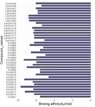
classes of quorum sensing inhibitors have been synthesized and tested through cell-based assays to
42
evaluate how well they perform at limiting bacterial congregation. A different class of multi-aromatic
43
molecules, indoles, are known to modulate the quorum signaling response [5]. Indoles behave
44
similarly to N-acyl homo-serine lactones, due to their having much of the same structural, chemical
45
and topographic features. An observation that could be easily seen by medicinal chemists is the
46
common presence of the amide bonded to a cyclic ring. Shown in Table 1are examples of these
47
compounds, while a full list of relevant structures can be found in the Appendix A.
48
Table 1. Examples of quorum sensing inhibitors
49
Compound structure Compound Name Source
N-heptanoyl-L-homoserine
lactone Geske [4]
N
-(2-Methyl-1H-indol-5-yl)hexanamide Nath [5]
The present study uses computational ligand-receptor docking data in tandem with machine
50
learning algorithms to uncover design rules for quorum sensing chemical systems. Quantitative
51
structure-activity relationship (QSAR) methods produce a large set of numerical descriptions for the
52
chemical space that is desired. Medicinal chemists use these descriptors to interpret functional
53
differences in structurally similar compounds [6]. Using the R statistical language and the caret
54
machine learning package, these descriptor values will be processed for importance, and passed into
55
a neural network for training and testing [7-8]. These neural networks are tuned,with other functions
56
in the caret package, to predict how well these molecules bind to the target protein. The predicted
57
modeling data will then be validated by a more computationally rigorous docking investigation. The
58
models generated using QSAR descriptors are then tuned for the discovery of design rules that may
59
aid as foundational new knowledge for discovering functional chemical spaces having the ability to
60
control or modulate the biofilm response.
61
2. Materials and Methods
63
A set of 37 molecules with known quorum sensing inhibition activity were selected from several
64
literature sources [4-5]. Two-dimensional structures of these molecules were constructed in
65
ChemDraw [9]. The two-dimensional files were converted to three-dimensional structure files using
66
OpenBabel, an open source molecular file converter [10]. Mol2 and PDBQT files were used as input
67
for QSAR descriptor calculation and molecular docking simulations, respectively. Structures of these
68
molecules can be found in Appendix A, while structure files can be found in the online supplemental
69
information.
70
The mol2 files of the compounds were input into DRAGON 7, a software that allows users to
71
calculate all structure-activity related descriptors for given three-dimensional structures [11]. This
72
software generated a table of comma separated values of the compounds and the values of all five
73
thousand seven hundred and seventy-two descriptors calculated.
74
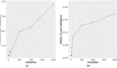
A crystalized protein structure of the LasR protein was found in the online protein data base
75
from a crystallography study and downloaded from the online protein data base in the form of a
76
PDBQT file [12-13]. Using autogrid4, the active site of the protein was visualized to assess the docking
77
ability of all quorum sensing inhibitor candidates [14]. Using AutoDock, a binding simulation
78
software, all inhibitors were docked in the active site of the LasR protein and spatially evaluated for
79
computation of the binding affinity of the protein-inhibitor interaction [15]. Figure 2 shows the
80
binding site that was evaluated in AutoDock.
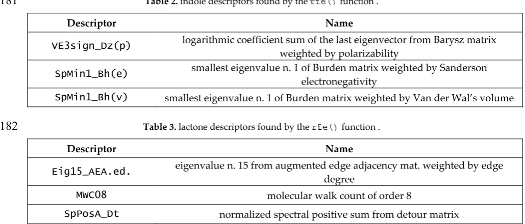
81
82
83
Figure 2. Figure of docking simulation between N-heptanoyl-L-homoserine lactone and the LasR
84
complex [11]
85
The binding affinity represents how well each compound fits to the active site of the protein,
86
which is a good predictor of how the interaction triggers a transcription event that regulates the
87
biofilm response. The values of binding affinities generated can be found in Appendix B. Since these
88
molecules successfully inhibit the protein by out-competing the natural ligand, the binding activity
89
is a negative value. The binding affinity of these interactions were computed and can be seen in
90
Figure 3. Binding affinity has units of kilojoules per mole and refers to the free energy liberated in
91
the binding interaction between ligand and receptor. The negative affinity for the binding interaction
92
indole class has some outliers with a more negative and thus stronger binding affinity [5]. Figure 3
94
shows the ranges of binding affinity throughout the set of molecules.
95
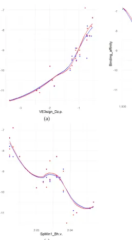
96
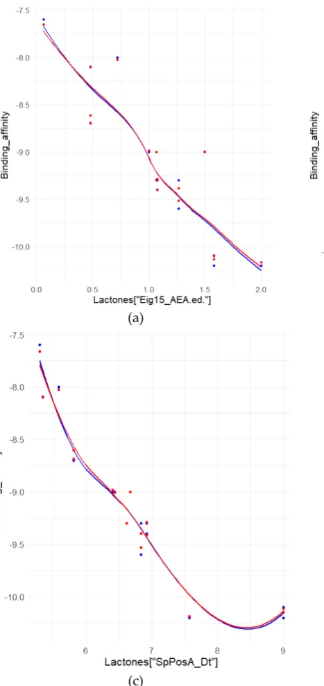
Figure 3. Bar graph of binding affinities calculated through AutoDock.
97
Binding affinities were appended onto the dataset of the QSAR descriptors for each molecule.
98
The dataset was saved as a table of comma separated values and read into a data frame using the R
99
statistical language. R was used to find important variables, wrangle data, explore different models,
100
test predictions, and to visualize data and models for evaluation of performance. The caret software
101
package is utilized to control and tune the models that are appropriate to our dataset. [8] The caret
102
software package, developed by Max Kuhn, allows users to choose from and adjust features of many
103
different of classification and regression models with machine-learning features. Scripts
104
demonstrating how these functions were implemented can be found in the online Supplemental
105
Material.
106
Initially, the dataset is split by molecule class using the nO descriptor, which is number of
107
oxygen atoms found in the molecule. The defining rule for descriptor split is that the lactone class
108
has one or two oxygen atoms, while the indole class has three or more oxygen atoms per molecule.
109
Separating these classes of molecules and having two different models allows for elucidation of
110
descriptors specific to each molecule class that drive the binding affinity of the molecule. Since the
111
own training and testing data. The createDataParition() function in caret allows for the
113
random splitting of data used to train and test neural networks. The argument p of the function is set
114
as 0.7, indicating that 70% of the molecules are used for training the networks, while the remaining
115
30% are used for validation of the model, ensuring that the model is learning about patterns of the
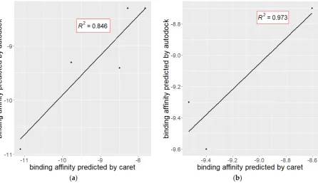
116
descriptor sets in the molecules.
117
To draw conclusions about which descriptors are integral for the functionality of the ligand
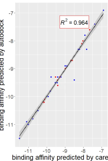
118
binding interaction, only relevant data should be considered for model input. Many QSAR studies
119
utilize numerical correlations or principal component analysis between each descriptor and its
120
binding to find which descriptors have predictive capabilities, but caret allows us to use other
121
options. A caret function called nzv() is used to drop the descriptor values that have near zero
122
variance between molecules. The nzv() function removes variables that are all 0 for the set of
123
molecules, thereby removing unimportant or uninformative descriptors. The recursive feature
124
elimination function, rfe(), in caret, is a backwards selection algorithm that uses a random forest
125
model to find the descriptors that serve as good predictors. In the rfe() function, multiple random
126
forest models are performed, and descriptors are ranked by their importance to the model. After each
127
iteration of the forest, the most important descriptors are retained and used to fit the next model. The
128
algorithm allows for selection of a specific number of descriptors for each molecule class.
129
QSAR and machine learning studies can use myriad different model-building algorithms such
130
as linear regression, random forests, support vector machines, and neural networks. Difference
131
between these models can be shown in the results subsection of this paper, Model Selection.Neural
132
networks are well-suited for QSAR studies because each descriptor can serve as an input to be
133
evaluated by the network. These inputs are used in multiple layers of functions utilizing linear
134
algebra to find the best function for the machine to learn how to predict binding affinity effectively.
135
For good model performance, it is important for each component of the model to be evaluated under
136
the condition of Bayesian methods [16]. Bayes’ rule is used to ensure that the statistical importance
137
of each descriptor is weighed independently, making models more robust and less prone to
138
overfitting [17].
139
The QSAR datasets are constrained to the important variables found from the rfe() and input
140
into a caret train object used to train a Bayesian-regularized neural network. Caret allowed for
141
quick tuning based on the number of neurons, weighting of variables at different points in the
142
network, amount of resampling, and cross-validation. To insure accuracy of these networks, each
143
neuron was input from a singular variable of a molecular descriptor. The output of these models is
144
the predicted binding affinities based on the QSAR descriptors. To validate the methodology, these
145
outputs can be compared to the binding affinity predicted by the docking simulation. The models,
146
once validated, allow for the elucidation of important structural and topographic features driving the
147
binding interaction.
148
3. Results
149
3.1 Model Selection
150
A variety of models can be used for QSAR, but some models are more ideal for appropriate for
151
characterization of the QS interaction. Caret allows for fast testing of different machine learning
152
models. Bayesian regularized artificial neural networks (BRANN) suit QSAR methodologies well due
153
to their reliance on individual descriptors. BRANNs tend to generalize features found in the
154
descriptions, creating more accurate predictions for the test data. Many QSAR-based machine
155
learning models rely on generalizing the dataset by though Bayesian methods for accurate prediction
156
of the molecular interaction of interest [17]. The QS activation of the LasR interaction can be modeled
157
through BRANNs. Figure 4 shows the statistical differences between each model establishing the
158
higher relative performance of BRANNs. These networks exhibited high performance through an
159
(a) (b)
Figure 4. (a)Model performance of the indoles set; (b) Model performance of the lactones set.
161
3.2 Descriptor Selection
162
The rfe()function was used to to differentiate performance of a molecule based upon their unique
163
set of molecular descriptors. To find the a proper size of descriptor set, a recursive function in R was
164
used to test how accuracy changes with the number of descriptors. Accuracy descreased with more
165
descriptors processed, and increased by focusing on the top twenty-five important descriptors. These
166
relationships can be seen in the Figure 5.
167
(a) (b)
Figure 5. RMSE increased observed though more descriptors analyzed by RFE (a) in the indoles set;
168
(b) in the lactones set.
169
Each class of molecules have different important descriptors identified by the rfe(). Many
171
descriptors are much more than simple counting observations such as how many oxygen atoms are
172
present in the molecule. Some descriptors are used to evalulate the topology of the molecules and
173
require matrix calculations. To explain what these desciptors mean, a brief overview of graph theory
174
is required. Graph theory is a mathematics approach to measure the edges and vertices of complex
175
geometries and can be applied in describing molecular structures [18]. In Chemical Graph Theory,
176
the authors explain how matrices can be used to estimate the distances between atoms and bonds in
177
the molecule. The topologies of the chemical structure have much to do with the conformations seen
178
in binding interactions as well their rigidity in these positions. Table 2 and 3 describe an index of
179
selected descriptors and their definitions.
180
Table 2. indole descriptors found by the rfe() function .
181
Descriptor Name
VE3sign_Dz(p) logarithmic coefficient sum of the last eigenvector from Barysz matrix weighted by polarizability
SpMin1_Bh(e) smallest eigenvalue n. 1 of Burden matrix weighted by Sanderson electronegativity
SpMin1_Bh(v) smallest eigenvalue n. 1 of Burden matrix weighted by Van der Wal’s volume
Table 3. lactone descriptors found by the rfe() function .
182
Descriptor Name
Eig15_AEA.ed. eigenvalue n. 15 from augmented edge adjacency mat. weighted by edge degree
MWC08 molecular walk count of order 8
SpPosA_Dt normalized spectral positive sum from detour matrix
Definitions of these descriptors rely on distance matrices used to measure the shape and topology.
183
Using Molecular Descriptors for Chemoinformaticsas a guidebook for these descriptors can serve as
184
assistance for understanding the descriptors. By observing the relationships between a molecule
185
binding and its structural motifs, description-based guidelines be generated to show non-intuitive
186
relationships. The molecules classified as indoles had important molecules descriptions that related
187
to binding, shown in the Figure 6.
188
(a) (b)
(c)
Figure 6. Relationships between binding affinity(kJ/mole) and molecular descriptions of the indoles
190
set based on the descriptor; (a) VE3sign_Dz(p); (b) SpMin1_Bh(e); (c) SpMin1_Bh(e); data appearing
191
in red was calculated by neural networks while data in blue was generated through AutoDock.
192
The relationship between descriptors and molecules tend to group the molecules in different
193
sets based on topographical features. Through deduction one can uncover generalized rules for
194
binding. The descriptor VE3sign_Dz(p) has a positive correlation with binding affinity while the
195
descriptors, SpMin1_Bh(e) and SpMin1_Bh(v) have a negative correlation with binding affinity
196
for the indole-type molecules.
197
198
199
Groupings of descriptor data that account for the high binding affinity characteristics of selected
201
molecules can be used to establish criteria for high-binding indoles. The criteria for high-binding
202
(a binding affinity below -9.5 kJ/mole) indoles is as follows;
203
• SpMin1_Bh(e) > 1.94
204
• SpMin1_Bh(v) > 2.03
205
• VE3sign_Dz(p) < -1.5
206
The same comparison between descriptors and binding affinity was made with the lactones data
207
and can be seen in Figure 7.
208
(a) (b)
(c)
Figure 7. Relationships between binding affinity(kJ/mole) and molecular descriptions of the lactones
209
set based on the descriptor; (a) Eig15_AEA; (b) MWC08; (c) SpPosA_Dt; data appearing in red was
210
The descriptors Eig15_AEA, MWC08, and SpPosA_Dt all have negative correlations with binding
212
affinity for the lactone-type molecules. Groupings of descriptor data that account for the high
213
binding affinity characteristics of selected lactones can be used to establish criteria like those
214
generated from the indoles set. The criteria for high-binding (a binding affinity below -9.5
215
kJ/mole) lactones is as follows;
216
• MWC08 > 9.5
217
• Eig15_AEA(ed) > 1.5
218
• SpPosA_Dt > 7.5
219
3.3. Neural Network Performance
220
BRANN models were trained with only 70% of the molecules and the test set of molecules were
221
used to validate model prediction. Results of the test set were computated with the
222
predict.train() function in caret, letting the model interpret new testing data for predictions
223
of new compounds. A comparison of the test values and predictions the model makes can be seen in
224
Figure 8. Values for predicted binding can be found in Appendix B.
225
(a) (b)
Figure 8, (a) Comparison of the indole set for validation of the its models prediction (R^2 = 0.875,
226
RMSE = 0.495, units in kJ/mole); (b) Comparison of the Lactone set for validation of the its models
227
prediction(R^2 = 0.873, RMSE = 0.189, units in kJ/mole)
228
One can also use the caret predict function to compare the training and testing set, to observe
229
results of predictions across the entire dataset. The comparison between all predictions can be
230
seen in Figure 9. Although this data in combined from 2 different models, it shows relative
231
233
Figure 9. Comparison all molecules (R^2 = 0.961, RMSE = 0.211, units in kJ/mole)
234
3.4. Guidelines for high-binding QSIs
235
While the criteria for high-binding QSIs seen in section 3.2 are good guidelines for machine learning
236
prediction of binding, functional design of these molecules involves structural guidelines. Figure 10
237
and 11 show structures of the high binding molecules from each class along with key structural
238
features of the molecules that contribute to their binding interaction with QS receptors.
239
240
242
Figure 11. Key structural features of lactone 4
243
4. Discussion
244
Machine learning techniques like BRANNs for QSAR datasets allow for quick identification of
245
the biochemical molecular design rules guiding complex protein interactions. Structural and
246
topographical data for molecules provide insight about their function, as well as the underlying
247
mechanisms of signaling events such as quorum sensing.
248
Quorum sensing research currently relies on culturing a model species in the laboratory and
249
testing how well new inhibitors change the genotype of the bacteria. The testing assay relies on a
250
fluorescent marker that is activated through expression of the reporter protein. While this
251
methodology measures the change directly, it does not account for the intricacies of real world
252
problems in inhibiting biofilms.
253
At the beginning of this project, we attempted to use results of fluorescent assays as our
254
dependent variable instead of binding affinity. Fluorescence results as seen in the work of Nath et al.
255
are a direct measure of how well the new genes are activated by QSIs [5]. While an assay
256
measurement is indeed a direct measure of the biochemical effect, each research group or set of source
257
data uses a different negative control for relative fluorescence, meaning that different results are not
258
comparable across studies, a key setback when attempting to discover unifying design rules and
259
generalized models of performance. Using binding affinities predicted in silico by AutoDock is useful
260
for comparing binding-based design to based design. Machine learning and
structure-261
based design are complementary tools for discovering new knowledge about binding interactions.
262
Bacteria use the QS signaling process as a common language and the syntax of this language is more
263
complex than what can be observed through biology methodologies and experimentation. The work
264
presented by So and Karplus represents one such attempt at applying high-throughput
265
methodologies in QSAR studies[18]. Molecules that improve meaning of the signaling language, like
266
indoles, should be compared to those of other classes, and other topologies. Screening for similar
267
protein interactions that bacteria share signaling processes for could prove effective at gaining
268
knowledge about other signaling cascades that regulate the bacterial genome.
269
Discovering new alternatives or designing functional improvements in biological systems is
270
hard. An extensive amount of time is spent designing methodologies, synthesizing new molecules,
271
and analyzing results. The work presented in this study shows one such attempt at apply design tools
272
towards the discovery of guidelines for strong QSIs. Knowing this information, it enables more
273
conclusions to be drawn about QS solutions for fighting biofilms.
274
Acknowledgments: This work was supported in part through the Bill and Linda Frost Fund at Cal Poly San Luis
276
Obispo. B.S. was selected as a Frost Research Fellow in the Frost Summer 2017 Undergraduate Research
277
Program.
278
Author Contributions: B.S. and E.S. designed the experiment; B.S. wrote scripts and performed analysis; E.S.
279
contributed software and knowledge; B.S. wrote the paper; B.S. and E.S. edited the paper.
280
Conflicts of Interest: The authors declare no conflict of interest.
281
282
283
284
285
286
287
288
289
290
291
292
293
294
295
296
297
298
299
300
301
302
303
304
Appendix A
306
Compound structure Reference Name
IUPAC Name
Source
Indole1 (11a)
N-(2-Phenyl-1H-indol-3-yl)
dodecanamide Nath [5]
Indole2 (11b)
N-(2-Phenyl-1H-indol-3-yl)
decanamide Nath [5]
Indole3 (11c)
4-Phenyl-N
-(2-phenyl-1H-indol-3-yl) butanamide Nath [5]
Indole4
(11d) N-(2-Phenyl-1H-indol-3-yl) hexanamide
Nath [5]
Indole5 (11e)
3-(1H-indol-3-yl)-N -(2-
phenyl-1H-indol-3-yl)propanamide
Nath [5]
Indole6 (14a)
3-Oxo-N
-(2-phenyl-1H-indol-3-yl)dodecanamide Nath [5]
Indole7 (14b)
3-Oxo-N
-(2-phenyl-1H-indol-3-yl)octanamide Nath [5]
Indole8 (14c)
3-Oxo-6-phenyl-N -(2-
phenyl-1H-indol-3-yl)hexanamide
Nath [5]
Indole9 (16a)
N
Compound structure Reference Name
IUPAC Name
Source
Indole10
(16b) N-(2-Methyl-1H-indol-5-yl)decanamide Nath [5]
Indole11 (16c)
N
-(2-Methyl-1H-indol-5-yl)-4-phenylbutanamide Nath [5]
Indole12 (16d)
N
-(2-Methyl-1H-indol-5-yl)hexanamide Nath [5]
Indole13
(16e) 3-(1H-Indol-3-yl)-Methyl-1H-indol-5-N
-(2-yl)propanamide
Nath [5]
Indole14 (17a)
N
-(2-Methyl-1H-indol-5-yl)-3-oxododecanamide Nath [5]
Indole15 (17b)
N
-(2-Methyl-1H-indol-5-yl)-3-oxodooctanamide Nath [5]
Indole16 (17c)
N
-(2-Methyl-1H-indol-5-yl)-3-oxo-6-phenylhexanamide Nath [5]
Indole17 (19)
1H-Indol-7-amine
Nath [5]
Indole18 (20a)
N
Compound structure Reference Name
IUPAC Name
Source
Indole19
(20b) N -(1H-Indol-7-yl)hexanamide
Nath [5]
Indole20
(20c) Nphenylbutanamide -(1H-Indol-7-yl)-4- Nath [5]
Indole21 (21a)
N
-(1H-Indol-7-yl)-3-oxododecanamide Nath [5]
Indole22 (21b)
N
-(1H-Indol-7-yl)-3-oxooctanamide Nath [5]
Indole23 (21c)
N
-(1H-Indol-7-yl)-3-oxo-6-phenylhexanamide Nath [5]
Lactone1 (7g)
N-heptanoyl-L-homoserine lactone
Geske [4]
Lactone2 (7h)
N -(indole-3-butanoyl)-L-homoserine lactone
Geske [4]
Lactone3 (7i)
N
-(indole-3-butanoyl)-D-homoserine lactone Geske [4]
Lactone4 (7j)
N-Boc-(4-aminomethyl)-N -benzoyl-L-homoserine
lactone
Compound structure Reference Name
IUPAC Name
Source
Lactone5 (7k)
N -(2-cyclo-entene-1-acetonoyl)-L-homoserine
lactone
Geske [4]
Lactone6 (7l)
N -(2-cyclo-entene-1-acetonoyl)-D-homoserine
lactone
Geske [4]
Lactone7 (7m)
N -Boc-aminocapranoyl-L-homoserine lactone
Geske [4]
Lactone8
(7n) N-monoethyl fumaroyl-L-homoserine lactone Geske [4]
Lactone9 (7o)
N
-(4- bromophenylacetanoyl)-L-homoserine lactone
Geske [4]
Lactone10 (7p)
N-(trans- cinamoyl)-L-homoserine lactone
Geske [4]
Lactone11 (7q)
N
-(4-phenylbutanoyl)-L-homoserine lactone Geske [4]
Lactone12 (7r)
N
-(4-phenylbutanoyl)-D-homoserine lactone Geske [4]
Lactone13 (8f)
N -(3-oxo-3-
phenylpropanoyl)-L-homoserine lactone
Geske [4]
Lactone14 (8g)
N -(3-oxo-3-
phenylpropanoyl)-D-homoserine lactone
Compound structure Reference Name
IUPAC Name
Source
Lactone15 (8h)
N
-(3-oxo-3-octanoyl)-D-homoserine lactone Geske [4]
Lactone16 (9)
N-
(2-Hydroxyphenyl)-3-oxooctanamide Geske [4]
307
Appendix B
308
Reference Name Binding Affinity predicted by autodock( kJ/mole)
Binding Affinity predicted by
caret( kJ/mole)
Indole1 -8.3 -8.302988
Indole2 -8.3 -7.988344
Indole3 -8.9 -8.937417
Indole4 -7.4 -7.417268
Indole5 -9.8 -9.795367
Indole6 -8.3 -8.325539
Indole7 -7.8 -7.851770
Indole8 -10.0 -9.936407
Indole9 -9.3 -9.377961
Indole10 -9.3 -9.253377
Indole11 -10.8 -10.831108
Indole12 -9.4 -8.554745
Indole13 -11.5 -11.433772
Indole14 -9.3 -9.988707
Indole15 -9.5 -9.494719
Indole16 -10.9 -11.448594
Indole17 -6.9 -6.926807
Indole18 -9.0 -9.035383
Indole19 -8.3 -8.280500
Indole20 -10.5 -10.444431
Indole21 -9.5 -9.462499
Indole22 -8.9 -8.951946
Indole23 -11.0 -10.992407
Lactone1 -7.6 -7.64831
Lactone2 -10.1 -10.118163
Lactone3 -10.2 -10.138430
Reference Name Binding Affinity predicted by autodock( kJ/mole)
Binding Affinity predicted b
y caret( kJ/mole)
Lactone5 -8.7 -8.583115
Lactone6 -8.7 -8.678089
Lactone7 -9.0 -8.990841
Lactone8 -8.1 -8.103228
Lactone9 -9.0 -9.013618
Lactone10 -9.3 -9.310404
Lactone11 -9.3 -9.272423
Lactone12 -9.4 -9.425550
Lactone13 -9.3 -9.487820
Lactone14 -9.6 -9.460026
Lactone15 -8.0 -8.043582
Lactone16 -9.0 -8.979812
309
References
310
1. Bakke, R.; Kommedal, R.; Kalvenes, S. Quantification of biofilm accumulation by an optical
311
approach. J. Microbiol. Methods 2001, 44, 13–26; DOI: 10.1016/S0167-7012(00)00236-0.
312
2. Soulère, L.; Marine F.; Yves Q.; Alain D. Exploring the Active Site of Acyl Homoserine
Lactones-313
Dependent Transcriptional Regulators with Bacterial Quorum Sensing Modulators Using
314
Molecular Mechanics and Docking Studies. Journal of Molecular Graphics and Modelling. 2007,
315
581–590; DOI: 10.1016/j.jmgm.2007.04.004.
316
3. Ni, N.; Minyong L.; Junfeng W.; and Binghe W. Inhibitors and Antagonists of Bacterial Quorum
317
Sensing. Medicinal Research Reviews, 2009. 65-154; DOI:10.1002/med.20145.
318
4. Geske, G.D.; Rachel J.W.; Adam P.S.; and Helen E.B. Small Molecule Inhibitors of Bacterial
319
Quorum Sensing and Biofilm Formation. Journal of the American Chemical Society, 127, 2005,
320
12762–63; DOI:10.1021/ja0530321.
321
5. Nath, B.N.; Kutty, S.K.; Barraud, N.; Iskander, G.M.; Griffith, R.; Rice, S.A.; Willcox, M.; Black,
322
D.S.; Kumar, N. Indole-Based Novel Small Molecules for the Modulation of Bacterial Signaling
323
Pathways. Org. Biomol. Chem. 13, 3, 2015. 925–37. DOI:10.1039/C4OB02096K.
324
6. Mitchell, J. B. Machine Learning Methods in Chemoinformatics. Wiley Interdisciplinary Reviews:
325
Computational Molecular Science 4, 5, 2014. 468–81. DOI:10.1002/wcms.1183.
326
7. R Core Team. R: A language and environment for statistical computing. R Foundation for
327
Statistical Computing, 2007 Vienna, Austria. https://www.R-project.org
328
8. Kuhn, M.; Wing, J.; Weston, S.; Williams, A.; Keefer, C.; Engelhardt, A. Caret: Classification and
329
Regression Training. https://Cran.R-Project.Org/Package=Caret, 2012.
330
DOI:10.1053/j.sodo.2009.03.002.
331
9. Perkin Elmer Informatics, Chemdraw, 2012
332
10. O’Boyle, N.M.; Banck, M.; James, C.A.; Morley, C.; Vandermeersch, T.; Hutchison, G.R.; Open
333
Babel: An Open Chemical Toolbox. Journal of Cheminformatics 3, 10 2011.
DOI:10.1186/1758-2946-334
11. Andrea, M.; Consonni, V.; Pavan, M.; Todeschini, R. Dragon software: An easy approach to
336
molecular descriptor calculations. Match 56, 2, 2006. 237-248.
337
12. Zou, Y.; Nair, S.K. LasR-OC12 HSL Complex. PDB ID: 3IX3 TO BE PUBLISHED, n.d.
338
DOI:10.2210/PDB3IX3/PDB.
339
13. Berman, H.M.; Westbrook, J.; Feng, Z.; Gilliland, G.; Bhat, T.N.; Weissig, H.; Shindyalov, I.N.;
340
Bourne P.E. The Protein Data Bank Nucleic Acids Research, 28: 2000. 235-242.
341
14. Morris G.M.; Dallakyan, S. AutoDock.02-27 1, 2013. 15–45.
342
15. Trott, O.; Olson. A.J. AutoDock Vina. J. Comput. Chem. 31 2010. 445–61. DOI:10.1002/jcc.21334.
343
16. MacKay, D. J. C. A Practical Bayesian Framework for Backprop Networks. Neural Comput. 4
344
1992. 415-447
345
17. Winkler, D.A. The Role of Quantitative Structure--Activity Relationships (QSAR) in
346
Biomolecular Discovery. Briefings in Bioinformatics 3, 2002. 73–86. DOI:10.1093/bib/3.1.73.
347
18. Estrada, E.; Bonchev, D. Chemical Graph Theory. 1538-1558. 10.1201/b16132-92.
348
19. So, S.S.; Karplus, M. Evolutionary Optimization in Quantitative Structure-Activity Relationship:
349
An Application of Genetic Neural Networks. Journal of Medicinal Chemistry 39 1996. 1521–30.
350
DOI:10.1021/jm9507035.
351
20. Todeschini, R.; Consonni, V.; Mannhold, R.; Kubinyi, H.; Folkers, G. Molecular Descriptors for
![Figure 2. Figure of docking simulation between N-heptanoyl-L-homoserine lactone and the LasR complex [11]](https://thumb-us.123doks.com/thumbv2/123dok_us/7900935.1311562/3.595.136.466.367.617/figure-figure-docking-simulation-heptanoyl-homoserine-lactone-complex.webp)