Algorithmic Enhancements to the VULCAN Navier-Stokes Solver

(1)

Abstract

LITTON, DANIEL Algorithmic Enhancements to the VULCAN Navier-Stokes Solver. (Under the direction of Dr. Jack R. Edwards.)

(2)

Algorithmic Enhancements to the VULCAN

Navier-Stokes Solver

by

Daniel Litton

A thesis submitted to the Graduate Faculty of North Carolina State University

in partial fulfillment of the requirements for the Degree of

Master of Science

Aerospace Engineering

Raleigh, North Carolina 2003

Approved By:

____________________ _________________________

(3)

Biography

(4)

Acknowledgments

I would like to thank my parents who have been there for me every step of the way through my whole education, always pushing me to go farther. I would love to thank my loving wife, who has been very understanding and supportive throughout every stage of my education at North Carolina State University.

I would like to thank my advisor, Dr. Jack R. Edwards, for his guidance and support throughout my masters. Through him I was able to gain a great deal of knowledge concerning CFD and advice for the future. The instruction from my other committee members, Dr. D. Scott McRae and Dr. Ashok Gopalarathnam has been instrumental in my success as a graduate student. I would like to also thank them for their serving on my committee.

I definitely would like to thank everyone in Broughton 4216 for their help and useful discussions over the past two years.

I would like to thank NASA Langley for supporting this research under grant NAG-1-02052. I would like to thank Jeff White for his support and guidance while working at NASA Langley.

(5)

List of Figures

Figure 1: Example of decomposition of flat-plate ...52

Figure 2: Computational grid for West-Korkegi intersecting-wedges ...52

Figure 3: Computational grid for channel-flow...53

Figure 4: Convergence of planar relaxation scheme...53

Figure 5: Effect of CFL number on convergence ...54

Figure 6: Effect of sweep direction on convergence ...54

Figure 7: Effect of subiteration number on convergence...55

Figure 8: CPU time required versus number of subiterations...55

Figure 9: Effect of subiteration on subsonic channel-flow convergence...56

Figure 10: Condition number versus Mach number ...56

Figure 11: Computational grid for flow over a bump...57

Figure 12: Convergence history for various Mach numbers for flow over a bump ...57

Figure 13: Computational grid for flow over a flat-plate ...58

Figure 14: Convergence history for various Mach numbers for laminar flow over a flat-plate ...58

Figure 15: Convergence history for various Mach numbers for a turbulent, calorically perfect flow over a flat-plate...59

Figure 16: Convergence history for various Mach numbers for a turbulent, two-species air flow over a flat-plate...59

Figure 17: Convergence history for various Mach numbers for laminar flow over a flat-plate at a Reynolds number of 1.11×107...60

Figure 18: Convergence history for various Mach numbers for a turbulent, calorically perfect flow over a flat-plate at a Reynolds number of 1.11×107...60

Figure 19: Convergence history for various Mach numbers for a turbulent, two-species air flow over a flat-plate at a Reynolds number of 1.11×107...61

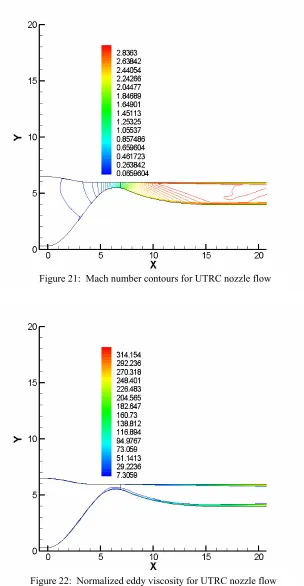
Figure 20: Computational grid for UTRC nozzle flow...61

Figure 21: Mach number contours for UTRC nozzle flow...62

Figure 22: Normalized eddy viscosity for UTRC nozzle flow ...62

Figure 23: Convergence histories: elliptic part of UTRC nozzle calculation...63

Figure 24: Convergence history for various Mach numbers for laminar flow through West-Korkegi intersecting-wedges ...63

(7)

intersecting-wedges...64 Figure 27: Convergence history for various Mach numbers for laminar

flow through West-Korkegi intersecting-wedges at a

Reynolds number of 1.11×107...65 Figure 28: Convergence history for various Mach numbers for laminar

flow through a channel...65 Figure 29: Convergence history for various Mach numbers for a

turbulent, calorically perfect gas flow through a channel...66 Figure 30: Convergence history for various Mach numbers for a

turbulent, two-species air flow through a channel ...66 Figure 31: Comparison of preconditioned system with non-preconditioned

(8)

List of Tables

(9)

List of Symbols

a Speed of sound

2 1

a Preconditioned interface sound speed

C Condition number

p

C Specific heat at constant pressure

i

D Diffusion coefficient of species i j

x

D_φ Modeled turbulent diffusion

C

E Convective contribution to the flux

I

E Interface flux

P

E Pressure contribution to the flux

t

E Total energy per unit volume G

F,

E, Flux vector

v v v ,F ,G

E Viscous flux vector

v v v f g

e , , Components of the viscous energy flux

h Enthalpy per unit mass

H Total enthalpy

k j,

i, Grid locations representing x, y, and z directions

J Jacobian

K Cutoff scalar

k Turbulent kinetic energy

l Iteration number

M Mach number

L

M~ , M~_R Left and right Mach numbers

ref

M Reference Mach number

i

M Molecular weight of species i

n Time level

±

R L

P_, Subsonic pressure splitting

T l,Pr

Pr Laminar and turbulent Prandtl number

p Pressure

z y x,q ,q

q Total heat flux vector

(10)

x

Re Reynolds number at distance x from leading edge

S Source term

T

c c S

S , Laminar and turbulent Schmidt number

T Temperature

( )

_p 1 k p k ,T

T − Preconditioned modal matrix

t Time

t

∆ Time step

w v,

u, Cartesian velocity components

d d d _,_v _,_w

u Cartesian diffusion velocity component W

V,

U, Contravariant velocity components

d d d _,_V _,_W

U Contravariant diffusion velocity components

R L ,U

U Left and right state at cell interface ∞

V Freestream velocity

ref

V Reference velocity

z y,

x, Cartesian coordinates

i

Y Mass fraction of species i

ζ η

ξ, , Transformed coordinates

t

µ

µ, Laminar and turbulent viscosity

λ Eigenvalue

c

ξ, p

λ Eigenvalue of the preconditioned Euler system

v

ξ, p

λ Viscous eigenvalue of the preconditioned Navier-Stokes system

κ Parameter to choose higher order schemes Φ Parameter to choose first order scheme

ψ Limiter

χ Thermal conductivity

ω Turbulence frequency

ρ Density

ij

τ Viscous stresses

(11)

1 Introduction

(12)

spacing. Convergence rates can degrade rapidly for highly-stretched meshes. Due to the lack of strong coupling between adjacent blocks, convergence rates are further degraded when large numbers of blocks are used.

Part of the present effort is concerned with improving the numerical efficiency of VULCAN for viscous flows on multi-block, highly-stretched meshes. Planar relaxation based implicit methods are introduced, along with sub-iterative procedures that allow for a large degree of implicit coupling among blocks. The implicit algorithm is an important aspect of eliminating convergence problems created by using multiple blocks. In order to accomplish this, the algorithm takes advantage of the MPI message-passing implemented in VULCAN. MPI message-passing is used to adapt VULCAN to parallel architectures by allowing necessary information to be passed between processors. With this new algorithm in place, it is expected that the convergence of most, if not all problems, will be greatly improved. It will be proven that the benefits of the new algorithm will outweigh the extra calculation time required in implementing this algorithm, at least for the problems tested.

(13)

(14)

airfoil flying in the transonic region that contains an area of low speed flow at the stagnation point.

To eliminate the need to have a different solver for low and high speed flows, it has become important to find one solver that would combine the best features of the “pressure-based” and “density-based” codes. The major issue that needs to be addressed is the disparity in the eigenvalues at low speeds. For a low speed flow, the magnitude of the convection speed is much lower than the acoustic speed. Due to the magnitude difference of the convection and acoustic speeds, the eigenvalues of the Euler equations (u,u+a,u−a) vary greatly from one another. This disparity in the eigenvalues is what causes the system to become very stiff. There are currently many solutions available to address this issue for compressible and incompressible flow solvers of all types. One of the first attempts [2] introduced an artificial time derivative of pressure into the continuity equation. With this artificial time derivative in place, it is now possible to advance the solution of the pressure field. Also, this term contains a parameter that serves to condition the eigenvalues to the same magnitude as the convection speed. This term is designed to vanish when the flow reaches steady state. This method, termed the Artificial Compressibility Method, was first introduced by Alexandre Chorin in 1967. [2] This artificial time derivative is placed only in the continuity equation and is given by

0 1

2 =

  

 

∂ ∂ + ∂ ∂ + ∂ ∂

y v x u t

p

(15)

for 2-D, incompressible flows. The term t p V_ref ∂

∂

2

1

is the artificial time derivative that

will vanish at steady state. The reference velocity, V_ref , is typically set to a multiple of the maximum flow velocity. Since the initial equation set is formulated for the incompressible Navier-Stokes equations, this derivation will not work for compressible flows without additions.

Although Chorin’s preconditioner only works for low speed, nearly incompressible flows, it can be extended to work for compressible flows. Currently, there are many different methods available to extend compressible solvers to low speed flows. [3] [4] [5] The preconditioner in VULCAN is that of Weiss and Smith [5]; however, it is formulated for conservative variables, rather than primitive variables. Their formulation has been proven to work for flows of all speeds.

According to Weiss and Smith, the artificial time derivative needs one major change in order to work for compressible flows. The equation set needs to have the ability to revert back to the compressible equations as the compressible limit is reached. This is accomplished by the addition of a parameter similar to Chorin’s to all equations in the compressible Navier-Stokes equation set. As before, this parameter will help the system to maintain good conditioning of the eigenvalues for low speed flows. The continuity equation with the addition of this parameter is defined as

( ) ( )



(16)

The parameter

t p a V_ref ∂

∂     

  

− ₂

2

1 1

is the additional term added to the continuity equation.

This term is derived as follows:

1. Chorin’s artificial time derivative,

t p V_ref ∂

∂

2

1

, is added to the continuity equation

2. The time derivative of density, t

∂ ∂ρ

is then subtracted from the continuity

equation in order to counter the effect of Chorin’s artificial time derivative 3. This time derivative of density is then converted to a time derivative of pressure

by means of the isentropic flow relations to produce

t p

a ∂

∂ 2

1

Once these changes are implemented, the altered continuity Equation 2 is formed. At low speeds (_V2 _a2

ref << ), Chorin’s artificial time derivative dominates, and the

eigenvalues become well conditioned. When V_ref2 is equal to a2, the whole term vanishes, and the original compressible equations are solved. Further derivation and discussion can be located in Section 4 after the necessary equations have been defined.

(17)

(18)

2 Governing Equations

2.1 Navier-Stokes equation set

VULCAN solves the three-dimensional Navier-Stokes equations, expanded to include separate transport equations for individual species and two-equation turbulence model components. The Navier Stokes Equations are written in a generalized coordinate system by the transformation:

(

)

(

)

(

x y z

)

z y x

, ,

ζ ζ

η η

ξ ξ

= = =

(3)

Written in this generalized coordinate system, the Navier-Stokes equations are given by

0 )

( =

+ ∂t R Q dQ

(4)

with the residual operator R(Q) given as

S G G F

F E

E Q

R v v v −

∂ − ∂ + ∂

− ∂ + ∂

− ∂ =

ζ η

ξ

) (

)

( (5)

(19)

                              = ρω ρ ρ ρ ρρ ρ ρ k Ew v u Y Y J Q t N_CS M 1 1 (6)

and the inviscid flux terms are defined as

(

)

                                + + + + ∇ = U kU U p E p Uw p Uv p Uu U U Y U Y J E t q y x N_CS ρω ρ ξ ρ ξ ρ ξ ρ ρ ρ ρ ξ M 1

(

)

                              ++ + + ∇ = V kV V p E p wV p vV p uV V V Y V Y J F t z y x N_CS ρω ρ η ρ η ρ η ρ ρ ρ ρ η M 1

(

)

                              ++ + + ∇ = W kW W p E p wW p vW p uW W W Y W Y J G t z y x N_CS ρω ρ ζ ρ ζ ρ ζ ρ ρ ρ ρ ζ M 1 (7)

(20)

(21)

with the source-term vector is given as                                 = ω ω ω ω S S J S k N i CS 0 0 0 0 1 & & M & (10)

In the above equations, Y_i is the mass fraction of the ith chemical species and

CS

N is the total number of chemical species. Also, p is the pressure, ρ is the density, v

u, and w are the Cartesian velocity components, E_tis the total energy, and the metric derivatives are defined as ξ_k,η_k,ζ_k. Finally, the turbulent terms, kand ω, are defined as the turbulent kinetic energy and the turbulence frequency. In the viscous flux vectors, τ_ij are the viscous stresses and e_v,f_v,g_v are the components of the viscous energy flux given by

(22)

      ∂ ∂ + ∂ ∂ =       ∂ ∂ + ∂ ∂ =       ∂ ∂ + ∂ ∂ = y w z v x w z u x v y u yz xz xy µ τ µ τ µ τ (12) and z z zz yz xz v y y yz yy xy v x x xz xy xx v D q w v u g D q w v u f D q w v u e φ φ φ τ τ τ τ τ τ τ τ τ + − + + = + − + + = + − + + = (13)

where the total heat flux and the modeled turbulent diffusion terms are defined as

∑

=       + − ∂ ∂       + − = CS j N i ij i ct t c j t t

x hY

S S x T q 1 Pr µ µ ρ µ

χ (14)

j t t l x x D _j ∂ ∂         + = µ µ φ φ φ

φ _Pr _Pr (15)

The subscript j represents the coordinate direction x, y, or z and φ represents either the k or ω turbulent equation. χrepresents the thermal conductivity. The terms µ and µ_t are defined as the laminar and turbulent viscosities, while Pr and _l Pr are the _t laminar and turbulent Prandtl number. S_c and S_ct are the laminar and turbulent

Schmidt numbers. Finally, the term " "

j iu u

(23)

ij ij k k i j j i t j i k x u x u x u u

u µ δ ρ δ

ρ 3 2 3 2 " " ₋         ∂ ∂ −         ∂ ∂ + ∂ ∂ =

− (16)

where

ω

µ_t = k (17)

The source terms S_k and S_ω are represented by

2 " " * " " βω ρ ω α ω β ρ ω _∂ − ∂ = − ∂ ∂ = j i j i j i j i k x U u u k S k x U u u S (18)

where the relations in the above equation are given from Wilcox [6] as

100 9 , 25 9 , , , 25 13 * 0 0 * 0 *

0 = * = =

=

= β β β β β β

α f_β f_β (19)

( )

_      ∂ ∂ − ∂ ∂ = Ω Ω Ω ≡ + + = i j j i ij ki jk ij x U x U S F 2 1 , , 80 1 70 1 3 * 0ω β χ χ χ ω ω ω

β (20)

j j k k k k k i j j i ij x x k f x U x U S ∂ ∂ ∂ ∂ ≡      > + + > =         ∂ ∂ + ∂ ∂ = ω ω χ χ χ χ χ β 3 2 2 1 0 , 400 1 680 1 0 , 1 , 2 1

* (21)

(24)

2 2 2

z y x ξ ξ

ξ

ξ = + +

∇ (23)

w v u

U =ξ_x +ξ_y +ξ_z , V =η_xu+η_yv+η_zw, W =ζ_xu+ζ_yv+ζ_zw (24)

The contravariant diffusion velocities are given by

d z d y d x

d _u _v _w

U =ξ +ξ +ξ d

z d y d x

d _u _v _w

V =η +η +η (25)

d z d y d x

d _u _v _w

W =ζ +ζ +ζ

where ud,vd, and wd are defined as the Cartesian diffusion velocities given by Fick’s law: i i i d Y x Y D u 1 ∂ ∂ = , i i i d Y y Y D v 1 ∂ ∂ = , i i i d Y z Y D w 1 ∂ ∂

= (26)

with D_i representing the diffusion coefficient of species i and

x Y_i ∂ ∂ the concentration gradient.

The Jacobian, J, of the transformation is defined as [7]

(

)

(

)

ζ η ξ ζ η ξ ζ η ξ ζ η ξ z z z y y y x x x z y x J J 1 , , , , 1 1 1 = ∂ ∂ =

= ₋ (27)

2.2 Equations for a calorically-perfect gas

(25)

pressure, total enthalpy, static enthalpy, specific heat at constant pressure, and total energy are given by

RT

p = ρ (28)

) (

2

1 _u2 _v2 _w2 h

H = + + + (29)

T C

h= p (30)

1 − =

γ

γR

C_p (31)

p H

E_t =ρ − (32)

where R is defined to be the gas constant (287 J / Kg-K for air).

2.3 Equations for a thermally-perfect gas

The equations for a multi-component, thermally-perfect gas are different from a single component, calorically perfect gas. For a thermally-perfect gas, the pressure, species enthalpy, and static enthalpy are formed by the expressions:

∑

=

= NCS

i i i u

M Y T R p

1

ρ (33)

dT C h

h T

T pi i

i = +

∫

0

0 ₍₃₄₎

(26)

where R_u is the universal gas constant (8314 J / kmol-K) and M_i is the species molecular weight. The specific heat and enthalpy are modeled with a polynomial curve fit based on the temperature from McBride et al [8], [9].

2.4 Boundary Conditions

The boundary conditions are specified for four different sets of conditions. Three of these are expressed for the Navier Stokes equations. The final set of boundary conditions is written for the Euler equations.

The first set of boundary conditions are set up for solving a supersonic flow. Customary of supersonic inflow boundary conditions, all variables are fixed, equal to the freestream quantities. All outflow boundaries are set up as a zeroth order extrapolation of all variables. Finally, the no-slip, adiabatic wall condition is maintained at every wall.

(27)

The third set of boundary conditions is required to solve for a laminar and turbulent flow of a thermally perfect, subsonic, gas. The main difference from the second set is that the characteristic equations are not coded for a thermally perfect gas. Rather, a zeroth-order extrapolation of the Riemann invariant is used to calculate the sound speed at the inflow, and the rest of the flow is solved from calorically perfect, isentropic relationships. As before, the variables are determined at the wall by ensuring that the no-slip, adiabatic wall condition is upheld.

(28)

3 Planar Relaxation Implicit Flow Solvers for Multi-Block

Domains

3.1 Algorithm

Typical computational geometries are extremely complex, requiring many mesh nodes to resolve sufficiently for an accurate solution. Resolution is frequently enhanced by decomposing the geometry into smaller pieces, called blocks. An example of such a grid-decomposition can be seen in Figure 1. This is an example of the decomposition of a flat-plate into 16 blocks, where blocks 1 and 16 are denoted in the figure. One or more blocks can be assigned to a processor in such a manner that the memory and storage requirements are distributed evenly. Through MPI message passing, each processor then shares the necessary information between blocks/processors that are adjacent in the domain in order to complete the calculations.

(29)

The RLX3D option in VULCAN is built around a planar relaxation scheme for solving the subdomain implicit problem and is designed to solve the complete (not parabolized) Navier-Stokes equations. The planar relaxation scheme is first set to solve the equations implicitly on each plane and then step to the next plane in the chosen direction and again solve the equations implicitly. The crossflow plane linear system is approximately solved using an incomplete LU decomposition procedure. Finally, the sweep, or step, may be block-specific in any of the desired directions:

ζ η

ξ, , .

The planar relaxation scheme is based upon solving the planar block-pentadiagonal system for each domain. Let the block septadiagonal system, A, be defined as [a,b,c, d,f, g,h], where a represents the linearization of the equation system at the point (i-1, j, k), b represents the linearization about point (i, j-1, k), c

represents the linearization about point (i, j, k-1), d represents the block diagonal, f represents the linearization about point (i, j, k+1), g represents the linearization about point (i, j+1, k), and finally, h represents the linearization about point (i+1, j, k). This implicit operator is then factored as

(

D a

) (

D D h

)

M = + −1 + ₍₃₆₎

where

(

d b c

) (

d d f g

)

D= ~+ + ~−1 ~+ + ₍₃₇₎

~ ~ ~ ~

− −

(30)

The system _M_∆_Qn+1 ₌₋_Rn_{is then solved by inverting the implicit operator,}_M _{. The} subdomain implicit operator, M , is inverted with a forward, then a backward sweep in the i direction as

Forward Sweep solving

(

_D₊_a

)

_∆_Q** ₌₋_Rn₍₃₈₎

1. solve - ** 1

(

₁

)

−

− ₋ ₋ _∆

=

∆Q_i D R_i a Q_i

Backward Sweep solving

(

_D₊_h

)

_∆_Q*** ₌_D_∆_Q**₍₃₉₎

1. solve - ***

1 1 * * *

* *

+

− _∆

− ∆ =

∆Q_i Q_i D h Q_i

This approach alleviates much of the numerical stiffness associated with highly-stretched mesh cells, provided that the crossflow plane contains the coordinate direction(s) with the largest degree of mesh stretching. Techniques such as Jacobian freezing and implicit boundary conditions are used to reduce the overall CPU load, and further enhance stability. Jacobian freezing is where the Jacobian matrices are reevaluated and re-factored after a certain number of iterations. In the cases presented, the Jacobian matrices are typically calculated, factored, and stored every iteration for the first 500 iterations, and then once every 5 iterations afterwards.

(31)

E N

M+ + , where N contains elements of A that would multiply corrections in adjacent subdomains and E is the factorization error. Given this, a general iterative scheme for improving the solution of the linear problem at a particular subdomain may be defined as:

l n n

l n l

n _Q _R _A _Q

Q

M₍_∆ +1,+1₋_∆ +1, ₎₌₋ ₋ _∆ +1, ₍₄₀₎

for _∆_Qn+1,l+1

Here, the index ndenotes a particular iteration level for the solution of the nonlinear problem (for unsteady flows, this could be part of another subiteration), and the index

l denotes a particular iteration level for the iterative improvement of the solution of the linear problem. With this basic strategy in place, one can define an algorithm for improving block-to-block coupling:

Solve: ∆Qn+1,1 =−M−1Rn (41)

For l=1, l_max:

1: Pass appropriate∆Qn+1,lelements to ghost cells of adjacent blocks (parallel MPI send / receive)

(32)

This algorithm requires that an extra block diagonal matrix, corresponding to the block diagonal ofA, which is normally over-written by the incomplete LU factorization, be stored in addition to M itself. The only change to the VULCAN input deck necessary to implement this algorithm is a flag indicating the number of subiterations performed,

.

max

(33)

4 Time-Derivative Preconditioning

4.1 Algorithm

The time-derivative preconditioning strategy currently implemented in VULCAN combines the rank-one preconditioning matrix of Weiss and Smith [5] with the “all-speed” version of the low diffusion flux-splitting scheme (LDFSS) of Edwards [10]. The “all-speed” version was developed according to a methodology presented in Edwards and Liou [11]. In order to complete the derivation of the Weiss and Smith preconditioning matrix begun in the introduction, it is necessary to make certain additions to the Navier-Stokes equation set. The first step in creating a more complete

system is to add a variant of the preconditioning term,

t p a

Vref ∂

∂     

  

− ₂

2

1 1

, to each

equation in the Navier-Stokes equation set. The additions are of the form t p uj

∂ ∂

θ for

the momentum equations and t p h

∂ ∂

θ for the energy equation, where θ is the scaling

parameter, 1₂ 1₂ a Vref

− . The next step is to take advantage of the fact that the pressure,

p, is a function of the conserved variables, Q, and can be expanded by the chain rule as

(34)

eq

N and q_i in Equation 44 represent the total number of equations and conserved variable, respectively. Once the expansion has been done, Equation 44 can be factored into a more suitable form:

t Q v t p T ∂ ∂ = ∂ ∂ (45) where         ∂ ∂ ∂ ∂ ∂ ∂ ∂ ∂ = Neq T q p q p q p q p

vr _K

3 2

1

(46)

With this addition, the two time derivative terms in Equation 2 (with the addition of the momentum, energy, and turbulence equations) can now be factored into one term as

(

)

t Q v u I t Q t Q v

u T T

∂ ∂ + = ∂ ∂ + ∂

∂ _r_r

r

r _θ

θ (47)

where urT, given by

[

Y Y u v w H k ω

]

urT = ₁ _K _N_CS 1 , (48)

represents the variants added to the momentum, energy, and turbulence equations. Finally, the preconditioned Navier-Stokes equation set with the additions from Equations 46-48 is given by

0 ) ( = + ∂ ∂ Q R t Q

P (49)

where the preconditioning matrix, P, is defined as

T

v u I

(35)

The reference velocity, V_ref , is responsible for scaling the eigenvalues of the equation set at low speeds to be of the same order. V_ref is defined as

   

 

   

 

= 2 2 _∞2

2 _min _a _,_max _V _,KV

V_ref r , (51)

where a is the sound speed and Vr2 is the velocity magnitude. V_∞ in the above equation acts as a cutoff velocity to prevent singularities in the proximity of stagnation regions. In the VULCAN implementation, the constant K scaling the cutoff velocity is a user input, and V_∞ is set to the inputted free-stream velocity.

The eigenvalues of

Q E P 1

∂ ∂

− _are:

U, U , U (52)

(

)

(

)

_



 ₊ _± ₋ ₊

=

± ₁ 2 2₁ 2 2 ₄ 2

2 1 '

' a M_ref U U M_ref V_ref

U (53)

where ₂

2 2

a V

M_ref = ref (54)

In the above equations, U is the contravariant velocity. As the incompressible limit is approached (V_ref2 → 0), the eigenvalues become

(36)

whereas the eigenvalues revert to their traditional values U,U,U, and U ±a as 2 ref

V

→a2. U in the above equations represents the contravariant velocity in the ξ

direction.

4.2 Numerical Discretization

To ensure accuracy at all flow speeds, it is necessary that the numerical discretization of the inviscid flux terms reflect the preconditioned eigensystem. In the VULCAN implementation, a preconditioned variant of the low diffusion flux-splitting scheme (LDFSS) of Edwards [10], developed according to a methodology presented in Edwards and Liou [11]. The interface flux E_I in LDFSS is split into convective and pressure contributions as follows:

[

L LC R CL

] [

p L L R R

]

I a C E C E E D p D p

E = ρ + +ρ − + + + −

2

1 (57)

The subscripts L and R denote the left and right states at the cell interface. The vector _EC_{is the same as}_ur _{in Equation 57, while}

[

0 0 0 _x _y _z 0 0 0

]

p

E = _K ξ ξ ξ (58)

The “preconditioned” interface sound speed

2 1

a is defined as

(

)

(

2

)

₁_/₂

2 / 1 2 2 2 2

1

4 1

2 1

ref

ref ref

M

V M

U a

+

  

 ₋ ₊

(37)

where the subscript ½ represents evaluation of the quantity using flowfield information arithmetically-averaged to the cell interface. The quantities D+, D−,C+, and C− are functions of left- and right-state Mach numbers, specially defined in terms of the interface sound speed and the reference Mach number as follows [11]:

  

 ₊ ₊ ₋

= _ref L _ref R

L M M M M

M (1 ) (1 )

2 1

~ 2

, 2

,

2 1 2

1 (60)

  

 ₊ ₊ ₋

= _ref _R _ref _L

R M M M M

M (1 ) (1 )

2 1

~ 2

, 2

,

2 1 2

1 (61)

with

2 1

/ ,

a U

MLR = L R (62)

The quantities D+, D−,C+, and C− are then given by

(

)

±

± ₌ ₊ ₋

R L R L R L R

L R

L P

D , α , 1.0 β , β , , (63)

(

)

+ +

+

+ ₌ ₊ ₋ ₋

2 1

1 M M M

C α_L β_L _L β_L _L (64a)

(

)

− −

−

− ₌ ₊ ₋ ₊

2 1

1 M M M

C αR βR R βR R (64b)

The definitions for the subsonic pressure splitting and the other functions are as follows

(

LR

) (

LR

)

R

L M M

P_, _, 1.0 2 2.0 _, 4

1

m ±

=

(38)

(

)

[

LR

]

R

L, 1.0 sgn M ,

2

1 _±

=

±

α (67)

For gas-dynamic flows, the use of the modified Mach number definitions in conjunction with the “preconditioned” sound speed enables the numerical dissipation mechanism of LDFSS to scale properly at all speeds. Exceptions to this are the definitions for C+and C−, which contain a pressure-dissipation term proportional to

R

L p

p − ,

      − − + − + =       − − + − − = − + R R L R L R L L R L R L R L p p p p p p p M M p p p p p p p M M δ δ 1 1 2 1 2 1 2 1 2 1 (68) where

(

~2 ~2

)

₁_.₀ 2

2 1 4 1 2 1       − +

= _L _R M_L M_R

M β β (69)

As shown in [11], this term acts to provide pressure-velocity coupling at low speeds, and to ensure that this effect scales properly, the term must be multiplied by _ref,2

2 1

1/M .

The primitive variables are extrapolated to the cell interfaces by means of the variable extrapolation scheme, MUSCL (Monotone Upstream-centered Schemes for Conservation Laws), of van Leer [12], given by

(

)

(

)

(

)

(

)

[

Q Q Q Q

]

Q

(39)

For values of Φ equal to 1, the MUSCL scheme is a higher order scheme, whereas Φ equal to zero results in a first order scheme. The scheme is second order accurate when κ is equal to 1₃_{and becomes Fromm’s second order scheme when}_κ

equals 0. All results in this paper are second order accurate, using κ equal to 13. In

order to ensure that no oscillations were present in the solution, the smooth limiter of Venkatakrishnan [13] was employed. Venkatakrishnan’s limiter is given by

( )

(

)

_

(

)

(

)

_ + + + + + + + = 11 4 3 4 , 1 4 11 1 3 4 min 1 2 1 2

2 _r _r

r r r r r r r

ψ (71)

After the addition of this limiter, the resulting scheme is

(

)

(

)

(

)

(

)

(

)

1

(

1

)

, , 1 2 , 1 , 2 2 1 2 1 2 1 2 3 2 3 2 3 2 1 1 1 1 4 1 1 1 4 − + − + − + − + + + − + − + − + + + −                     + +       − Φ + = −                     + +       − Φ − = i i i i i j i j i L i i i i i j i j i R u u r r r Q Q u u r r r Q Q ψ κ ψ κ ψ κ ψ κ (72) where 1 1 2 1 − + + − ₋ − = i i i i i _u _u

u u r 1 2 1 2 3 + + + − + ₋ − = i i i i

i _u _u

u u

r (73)

4.3 Time-Stepping Scheme

(40)

n Q

Q Q

Q F G S Q R

E t J P = ∆     ₊ ₊ ₊ ₋

∆ δξ δη δζ (74)

In Equation 74, EQ represents the Jacobian,

Q E Q E _v ∂ ∂ − ∂ ∂

and S_Q is defined to be

Q S ∂

∂ _.

The operator δ_ξE_Q∆Q is represented by

∆ξ ∆Q E ∆Q E 2 1 2 1 2 1 2

1 _i _Q_i _i

i

Q+ + − − −

(75)

where the interface states (_i₊₂1_{) are defined by an upwind approach such as}

1 2 1 2 1 2 1 2 1 ₊ − + + + +

+ ∆ i ≡ Qi ∆ i + Qi ∆ i

Qi Q E Q E Q

E (76)

where

(

)

2 1 2 1 1 , 2 1 − ±

+ ≡ E ±PTξ λ ξ Tξ

E_Qi _Q p c (77)

In Equation 77, the modal matrices, T_ξp and (T_ξp)−1, are constructed from diagonalization transformations of the form

Q E P T

Tp p c p

∂ ∂

= −

−1 1 , ( _ξ )

ξ

ξ λ (78)

where λpξ,c is a diagonal matrix containing the eigenvalues of the preconditioned Euler

(41)

( )

2

1 _t _O _t

t E E E n n

n _ _∆ ₊ _∆

     ∂ ∂ + =

+ ₍₇₉₎

where t Q Q E t Q Q E t

E n n n

∆ ∆       ∂ ∂ = ∂ ∂       ∂ ∂ =       ∂ ∂ +1

(80)

and after combining equations

( )

2

1 _Q _O _t

Q E E E n n

n _∆ ₊ _∆

      ∂ ∂ + =

+ ₍₈₁₎

After substituting Equation 81 into Equation 74 the result is

(

+ ∆

) (

+ + ∆

) (

+ + ∆

) (

− + ∆

)

=0

+ ∆ ∆ Q S S Q G G Q F F Q E E t J Q

P δ_ξ n _Q δ_η n _Q δ_ζ n _Q n _Q (82)

After rearranging and defining the steady state residual as

)

( n n n n

n _E _F _G _S

R =− ∂_ξ +∂_η +∂_ζ − (83)

the final equation becomes

(

) (

)

n

Q Q

Q

Q Q F Q G Q S Q R

E t

J Q

P + ∆ + ∆ + ∆ − ∆ =

∆ ∆

ζ η

ξ δ δ

δ (84)

(42)

[

]

[

(

)

]

[

(

)

]

(

)

[

]

n

k j i p v c p p p v c p p p v c p p Q R tP J Q T t J I T T t J I T T t J I T tS J I 1 , , 1 , , 1 , , 1 , , ) ( ) ( ) ( − − − − ∆ = ∆ − ∆ + − ∆ + − ∆ + ∆ − ζ ζ ζ ζ ζ η η η η η ξ ξ ξ ξ ξ λ λ δ λ λ δ λ λ δ (85)

and solved sequentially as

[

]

n

k j i

Q Q J tP R

tS J

I * 1

, , = ∆ − ∆ ∆ −

(

)

[

]

(

)

[

]

(

)

[

]

*** , , , , 1 , , * * , , * * * , , 1 , , * , , * * , , 1 , , ) ( ) ( ) ( k j i k j i p v c p p k j i k j i p v c p p k j i k j i p v c p p Q Q T t J I T Q Q T t J I T Q Q T t J I T ∆ = ∆ − ∆ + ∆ = ∆ − ∆ + ∆ = ∆ − ∆ + − − − ζ ζ ζ ζ ζ η η η η η ξ ξ ξ ξ ξ λ λ δ λ λ δ λ λ δ (86) k j i n k j i n k j

i Q Q

Q 1 _, _, _, _,

,

,+ = +∆

Again, _Tp

ξ and

( )

1 −

p

T_ξ are the modal matrices. An example of the modal matrices in one dimension for the preconditioned Euler system can be found in Appendix A. The diagonalizing procedure presented above relieves much of the expense involved with solving the system. The scheme reduces to solving a system of N scalar tridiagonals. Note that the first step of the DAF procedure is an approximation of the more exact expression

[

]

n

k j i

Q Q J tR

tS J

P− ∆ ∆ * = ∆

,

, (87)

(43)

u A v

A uv A A uv

A _T

T T

1 1 1

1 1

1 )

( ₋

− −

+ − =

+ (88)

This theorem applied to the preconditioning matrix above is given by

u v uv I uv

I

P _T

T T

+ − = +

= −

−

1 )

( 1

1 _θ ₍₈₉₎

The action of all other source Jacobian elements (those corresponding to chemistry and turbulence source terms) on the residual vector is computed in a separate step, involving the use of Householder transformations to ensure good numerical stability.

(44)

5 Results

5.1 Planar Relaxation Results

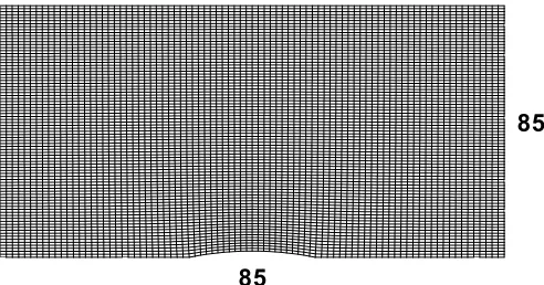
The testing of the planar relaxation algorithm with subdomain coupling has been focused on the West-Korkegi intersecting-wedge geometry [14] and a channel-flow analogue formed by eliminating the wedges and the clustering to the leading edge. The clustering in the Y and Z directions remains the same, as do the length, width, and height of the (now) rectangular geometry. Figures 2 and 3 portray the grid and dimensions used for the West-Korkegi intersecting-wedge geometry and the channel-flow grid. The free-stream conditions for the intersecting-wedge simulations are: M∞ =3, Re/m =2.11e6, T∞ =105 K. The free-stream conditions for the channel-flow simulations are: M∞ =0.5, Re/m =3.52e5, T∞ =105 K. In both cases, the grid size is 65x125x125 and laminar flow is assumed. Unless otherwise mentioned, all cases were performed in parallel on the North Carolina Supercomputing Center IBM-SP2 using a 16-block load-balanced decomposition of the baseline grid.

(45)

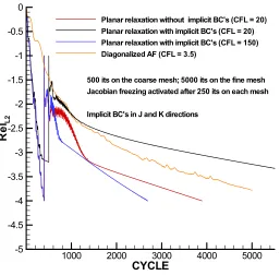
Figure 5 presents results from a CFL-ramping exercise performed for the supersonic West-Korkegi case. The final CFL number is reached by ramping from 0.1 to 20 over the first 500 iterations, from 20 to 150 over the next 500, and from 150 to the final value over the next 250 iterations. In this case and in most subsequent ones, the first 500 iterations are performed on a coarse mesh using a first-order accurate inviscid flux discretization. Jacobian freezing is initiated after 250 iterations, with re-evaluation and factorization of the matrices performed every 5 iterations past this point. The controlling parameter l_max is set to one for this study. Figure 6 shows that there is little advantage to choosing a CFL higher than 150 for this case. Figure 6 shows the effect of the choice of sweep direction on the performance of the iteratively improved planar relaxation algorithm with l_max= 0 and l_max=1. As anticipated, sweeping in the “i” direction (thedirection of the dominant movement of the supersonic flow) is clearly preferable to sweeping in the “j” direction. Performing one subiteration to improve the solution of the linear system improves the performance in both cases, at least in terms of the number of iterations.

(46)

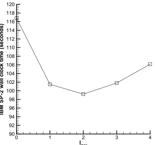
the trends are what one might expect. As the work increases significantly with the increase in the number of subiterations, it is instructive to examine wall clock time. Figure 8 shows that for this predominately supersonic flow, there is little benefit to performing the subiterations, with only about a 15% improvement in overall execution time for the best case of l_max= 2. Although the number of iterations decreases by almost half, the time spent in the subiteration loop erases some of the benefits from the scheme.

(47)

second-order case to the point that its convergence rate is very similar to the first-order case. Otherwise, as evidenced by the results, the second-order calculation eventually diverges. In comparison with the supersonic West and Korkegi case, these results indicate that the benefits of subiterative improvement of the linear system solution may be much larger for subsonic flows. The technique appears to aid in damping and/or expelling pressure disturbances that otherwise tend to reflect from physical and interface boundaries.

5.2 Preconditioning Results

The five test cases for the implementation of time-derivative preconditioning are the inviscid flow over a bump in a channel, flow over a flat-plate, flow through a two-dimensional United Technologies Research Center (UTRC) nozzle, flow between intersecting wedges, and finally, the flow through the channel analogue of the intersecting wedges. These correspond to variations on standard test cases included in the VULCAN package. In all cases the maximum CFL is set to 2.5 and the diagonalized approximate factorization scheme is used. Most cases involve both turbulent and laminar flow as well as multi-component gases. In all turbulent cases, the Wilcox (1998) k−ω model is used. For all cases involving multiple gas species, a mixture of nitrogen and oxygen is used.

(48)

min max

λ λ

=

C (90)

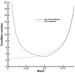
Figure 10 shows a direct correlation of the effect of the preconditioning of [11] on the condition number of the Euler equations. The disparity of the eigenvalues of the non-preconditioned system is readily apparent, while the preconditioned system demonstrates the desired correction to the Euler equations and eigenvalues. It is interesting to note that at approximately Mach 0.4, the eigenvalues of the non-preconditioned system appears to be slightly better conditioned than the non-preconditioned system.

5.2.1 Inviscid flow over a bump in a channel

(49)

5.2.2 Two-dimensional flow over flat plate

Figure 13 shows the 65x129 grid for the flat-plate simulation. The first run was used to compare the results of ramping the Mach number down from Mach 0.5 to Mach 0.005. The free-stream conditions for the Mach 0.5 simulation are given in Table 1. In each successive case the only parameter changed was the Mach number, which decreased the Reynolds number by a factor of 10 for each succeeding run. Figure 14 presents convergence histories for preconditioned and non-preconditioned laminar flow at each Mach number. Strikingly, it can be seen that the convergence of the non-preconditioned system is not altered by lowering the Mach number, whereas the preconditioned system converges faster for only Mach 0.5 and 0.05. A closer investigation into the solution produced by the non-preconditioned system verifies that the solution is in fact incorrect. The Blasius solution is calculated at distances of 0.3, 0.40, and 0.45 meters from the front edge of the flat plate. By using the Blasius solution for flow over a flat plate, the boundary layer thickness can be calculated as:

( )

x

x x

Re 0 . 5

=

δ (91)

(50)

Figures 15 and 16 show the results for a turbulent, calorically perfect and a turbulent, two-species air flow over a flat plate, respectively. The convergence histories for each case are very similar to that of the laminar flow in Figure 14. In all three examples, the preconditioned Mach 0.5 case shows a marked improvement in convergence over the non-preconditioned result. This is somewhat in contrast with the results from the eigenvalue analysis, which indicate that the non-preconditioned system should have a better overall condition number at this Mach number. One reason may be the presence, in the preconditioned flux-splitting, of pressure-diffusion terms that tend to smooth out variations in the pressure field. As will be seen in the next few examples, this result is independent of geometry. The convergence degradation indicated for the Mach 0.005 calculations could be associated with the decrease in Reynolds number. Stiffness due to low Reynolds numbers will not be alleviated by the inviscid preconditioning techniques currently employed in VULCAN.

As proof of this conjecture, a few cases were run holding the Reynolds number constant. The cases were all run at a Reynolds number of ₁_.₁₁_×₁₀7_{, the same as the}

(51)

convergence behavior. For the lower Mach number cases, the residual has almost converged to four orders of magnitude within 5000 iterations. Over 5000 iterations, the non-preconditioned residual only decreases a maximum of 2.5 orders of magnitude.

As can be seen by Figure 10, the condition number asymptotically goes down to 2.6 as the Mach number is lowered. Thus at lower Mach numbers it is expected that the convergence histories should be independent of Mach number. This is shown in Figure 18 for the turbulent flow of a calorically perfect gas. The convergence history for the Mach 0.05 and Mach 0.005 are nearly identical. Also, like the laminar case for the same Reynolds number, all three preconditioned cases converge much faster than their preconditioned counterparts. The convergence rate for the non-preconditioned system slows down as the Mach number is lowered.

(52)

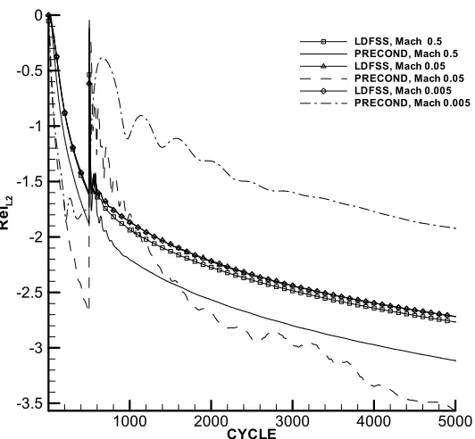
5.2.3 Two-dimensional flow through a nozzle

(53)

5.2.4 Three-dimensional flow through intersecting wedges

Figures 24-27 present results from simulations of subsonic viscous flow through the West-Korkegi intersecting wedge geometry (shown in Figure 2). Free-stream conditions are chosen to be the same as in the two-dimensional flat-plate case. Figure 24 illustrates the convergence histories for laminar flow through the wedges. The three non-preconditioned solutions do not converge at the same rate and show worse convergence than the preconditioned scheme at all Mach numbers, except Mach 0.005. As the Mach number decreases in magnitude beyond the Mach 0.5 case, the convergence rate is shown to decrease quickly. The preconditioned system contains a few oscillations but maintains its downward trend towards convergence. Figure 25 shows results for the turbulent, calorically perfect case. This case shows trends that are almost identical to the laminar flow.

The disparity in the results given by the non-preconditioned system is magnified when running the two species, turbulent simulation. As can be seen in Figure 26, the non-preconditioned residual at Mach 0.005 does not go down, but rather oscillates wildly around 10-1. Although its preconditioned counterpart does not display this behavior, the convergence rate is noticeably slowed down. The residual of the preconditioned system continues to go down towards convergence with minimal oscillations (in comparison to non-preconditioned system).

(54)

7

10 11 .

1 × . As expected, the preconditioned residual histories, shown in Figure 27, reveal a drastic improvement over the ones in Figure 24. The largest improvement can be seen when comparing the Mach 0.005 cases. In Figure 27, the residual has almost reached convergence at four orders of magnitude reduction; whereas in Figure 24 the residual has started leveling off around a 2.5 order of reduction in magnitude. The most striking feature in Figure 27 is the fact that the convergence history has become nearly independent of Mach number. As is readily apparent, the convergence histories for Mach 0.05 and Mach 0.005 are almost identical. This is expected due the condition number being virtually the same for both Mach numbers as seen in Figure 10.

5.2.5 Three-dimensional flow through a channel

The final case tested was the channel analogue of the West-Korkegi intersecting wedge geometry. Again, Figure 3 displays the computational grid used for the ramped Mach number simulations. Figure 28 shows the convergence histories for the ramped Mach number flows of a laminar flow through the channel. As previously observed, the preconditioned Mach 0.5 case converges faster than the non-preconditioned case. A notable difference is that there are more oscillations visible in the non-preconditioned residual histories that are not evidenced in the flat-plate solution.

(55)

preconditioned and non-preconditioned formulations versus the Blasius result. The boundary layer thickness obtained from the non-preconditioned formulation turned out to have an error of no less than 85%, while the preconditioned formulation provided results within a reasonable 6% of the theoretical values.

Figures 29 and 30 reveal how the convergence histories are affected by turbulent, calorically perfect and turbulent, thermally perfect two species air flow through the channel, respectively. Once more, the oscillations that were not present in the flat plate solution are very noticeable. Although these oscillations are present, both residual histories maintain their downward trend towards convergence.

(56)

6 Conclusions

(57)

7 Future Work

Future work will include the validation of the preconditioning model for low-speed reacting flows as well as implementing a change in the definition of the total enthalpy. Originally, the total enthalpy was defined as Equation 29, repeated below for convenience

(

2 2 2

)

2 1

w v u h

H = + + + (29)

This definition of the total enthalpy does not take into effect the turbulent kinetic energy parameter, k. Once this parameter has been added, the new total enthalpy becomes:

(

u v w

)

k

h

H = + 2+ 2 + 2 +

2 1

(92)

With this addition, a few terms are added to the modal matrices in Appendix A. The σ in Appendix A is representative of the modal matrix with and without the addition of the turbulent kinetic energy. Using σ equal to one represents the influence of the turbulent kinetic energy on the modal matrices. By using σ equal to zero, the matrix reverts back to its previous state.

(58)

References

[1] White, J.A. and Morrison, J.H., “A Psuedo-Temporal Multi-Grid Relaxation Scheme for Solving the Parabolized Navier-Stokes Equations,” AIAA 99-3360, July, 1999.

[2] A. J. Chorin, ‘‘A Numerical Method for Solving Incompressible Viscous Flow Problems,’’ J. of Computational Physics, Vol. 2, 1967, pp. 12-26.

[3] Choi, Y.H., and Merkle, C.L., “The Application of Preconditioning in Viscous Flows,” J. Computational Physics, Vol. 105, 1993, pp. 207-233.

[4] Turkel, E., “Preconditioned Methods for Solving the Incompressible and Low Speed Compressible Equations,” J. Computational Physics, Vol. 72, 1987, pp. 277-298.

[5] Weiss, J.M. and Smith, W.A., “Preconditioning Applied to Variable and Constant Density Flows,” AIAA Journal, Vol. 33, 1995, p. 2050.

[6] Wilcox, D. C., “Turbulence Modeling for CFD,” DCW Industries, (2000).

[7] Anderson, D. A., J.C. Tannehill and R.H. Pletcher, “Computational fluid mechanics and heat transfer,” Taylor and Francis, (1997).

[8] McBride, B.J., Heimel, S., Ehlers, J.G. and Gordon, S., “Thermodynamic

Properties to 6000 K for 210 Substances Involving the first 18 Elements,” NASA SP-3001, 1963.

[9] McBride, B.J., Gordon, S. and Reno, M.A., “Thermodynamic Data for Fifty Reference Elements,” NASA TP-3287, 1993.

[10] Edwards, J.R. “A Low-Diffusion Flux-Splitting Scheme for Navier-Stokes Calculations,” Computers & Fluids, Vol. 26, No. 6, 1997, pp. 635-659.

[11] Edwards, J.R. and Liou, M.-S. “Low-Diffusion Flux-Splitting Methods for Flows at all Speeds,” AIAA Journal, Vol. 36, No. 9, 1998, pp. 1610-1617.

(59)

[14] West, J.E., and Korkegi, R.H., “Supersonic Interaction in the Corner of

(60)

Appendix

A Modal Matrices

The modal matrices of the preconditioned Euler system are constructed from diagonalization transformations of the form

Q E P T

Tp pc p

∂ ∂

= −

−1 1

) ( λ

Based on the one dimensional equation set for a turbulent, two component gas, T and T-1 are given in Cartesian coordinates as

                        − + + − + + + + + = ρ ω ω ω ρ ρσ γ ρ γ ρ σ ρ ρ ρ ρ 0 0 0 0 0 0 0 1 1 2 0 0 0 0 0 0 0 0 1 0 0 0 0 0 0 0 0 2 2 2 2 1 1 1 B A kB kA k F uD GB E uC GA k u D uB C uA u B A B Y A Y Y B Y A Y Y T where

(

)

a a u a u A ' 2 ' '+ −

=

(

₂

)

' 2 ' ' a a a u u

B= − −

(

)

₂

[

(

₂

)

]

2 ' ' ' 2 1 ' ' R M a u a u a u a u C ρ − + − − + =

(

)

[

]

[

(

)

]

2 2 ' ' ' ' ' R M a a a u u a u u D ρ − − + − =

(

)

' 2 ' ' a u a u

E = + −

(

)

' 2 ' ' a a u u

F = − − _

     +

= u kσ

G

2

(61)

(

)

(

)

(

)

(

)

(

)

(

)

(

)

                                  − − − − − − − − − − − − − − − − − − − − − − = − ρ ρ ωρ ρ σ γ γ γ σ γ γ γ σ γ γ γ γ ρ ρ ρ ρ 1 0 0 0 0 0 0 1 0 0 0 0 0 1 1 1 0 0 0 1 1 1 0 0 0 1 1 1 2 1 1 0 0 0 0 0 0 1 0 0 0 0 0 0 1 2 2 2 2 2 2 2 1 1 k u M Mu Hu u L Lu

Hu a a a

u M Y Y T where

(

)

(

)

_   ₊ _± ₋ ₊ =

± ₁ 2 2₁ 2 2 ₄ 2

2 1 '

' a M_ref u u M_ref V_ref

u and ₂

2 2

a V M_ref = ref

2 1

− =γ

H

(

u a

)

u M a L ref − + = ' ' 2 2

(

)

u a u M a N ref − − == ' ' 2 2

The constant, σ, represents the effect of k, the turbulent kinetic energy parameter on the modal matrices. If σequals 1, the matrix includes the effect of k, whereas if σ

(62)

1

{

16

Figure 1: Example of decomposition of flat-plate

{

X Y

Z

65

125

(63)

X Y Z