Essentials of the macroscopic-microscopic folded-Yukawa approach and examples of its record in providing nuclear-structure data for simulations

Essentials

of

the

macroscopic-microscopic

folded-Yukawa

approach

and

examples

of

its

record

in

providing

nuclear-structure

data

for

simulations

Peter Möller1,⋆

1_{P.MollerScientificComputingandGraphics,Inc.,P.O.Box1440,LosAlamos,NM87544,USA}

Abstract. The macroscopic-microscopic model based on the folded-Yukawa

single-particle potential and a “finite-range” macroscopic model is probably the approach that has provided the most reliable predictions of alargenumber of nuclear-structure proper-ties forallnuclei between the proton and neutron drip lines. I will describe some basic features of the model and the development philosophy that may be the reason for its suc-cess. Examples of quantities modeled within the same model framework are, nuclear masses, ground-state level structure, including spins, ground-state shapes, fission barri-ers, heavy-ion fusion barribarri-ers, sub-barrier fusion cross sections,β-decay half-lives and

delayed neutron emission probabilities, shape coexistence, andα-decayQαenergies to

name a few. I will show how well it predicted various properties measuredafterpublished results. Rather than giving an incomplete model description here I will give a timeline of model development and provide references to typical applications and references that are sufficiently complete that several individuals have written computer codes based on these references, codes whose results have excellent agreement with ours.

1 Introduction

Most insight into and understanding of nuclear properties have historically and are currently obtained in terms of surprisingly simple models. In systems which depend mainly on electron behavior their properties can be obtained from solving the Schödinger equation with realistic, known Coulomb po-tentials. For the nuclear system with its up to a few hundred nucleons a many-body a Scrödinger equation with a potential based on the much more complicated nuclear forces cannot be solved in practice. Therefore other types of models are used. They are often referred to in a condescending manner as phenomenological, but, in a sense all “models” are phenomenological. We will here focus on the remarkable insights into nuclear properties that have been obtained by the “liquid-drop model”, the single-particle model and a combination of those, the “macroscopic-microscopic” method that still today is providing much insight about the properties of nuclei.

2 The liquid-drop model

The liquid-drop model has its origin in the semi-empirical mass model, usually attributed to von Weizäcker [1] and Bethe and Bacher [2]. In the liquid drop model the nuclear binding energy, which

Discrepancy (Exp. − Calc.) Calculated

Experimental

σth = 0.5595 MeV

FRDM (2012)

0 20 40 60 80 100 120 140 160

Neutron Number N − 10

0 10 0 10 0 10

Microscopic Energy (MeV)

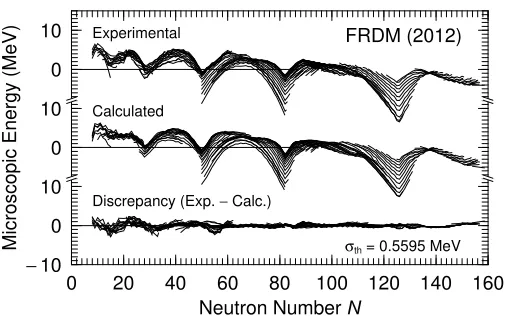
Figure 1.Comparison of

experimental and calculated microscopic energiesEmicfor 2149 nuclei, for a macroscopic model corresponding to the FRDM. The bottom part showing the difference between these two quantities is equivalent to the difference between measured and calculated ground-state masses. There are almost no

systematic errors remaining for nuclei withN≤65, for which region the error is only 0.355 MeV. The results shown in this figure represent our new mass model. The lines are drawn through isotope chains. From Ref. [6].

governs nuclear stability with respect toβandαdecay, is the sum of a volume energy term, due

to short-range “nuclear” forces, a Coulomb energy term due to the repulsive force between protons, a surface tension term, a symmetry energy term with its origin in the Pauli principle, and finally a pairing term.

B(N,Z)= +avA−asA2/3−aC Z

2

A1/3 −aI

(N−Z)2

A −δ(A) (1)

This simple expression gives the nuclear binding energy, which for a heavy nucleus is roughly 1600 MeV (8 MeV per nucleon) to an accuracy of one percent. The terms represent in order volume energy, surface energy, Coulomb energy, symmetry energy and a pairing correction. The notation Z, N, and Astand for proton number, neutron number and total nucleon number, respectively. It was highly useful in interpreting the decay chains following element transmutations. However, in some experiments in which uranium was bombarded with neutrons a confusing number of radioactive decay periods, which were difficult to reconcile with properties given by the semi-empirical mass model, were observed. This was all explained when Hahn and Strassmann [3] identified barium in the products following neutron irradiation of uranium and Meitner and Frisch [4] suggested one could think of the nucleus as a deformable charged liquid drop with a surface tension that had split into two smaller nuclei of about equal size in fission. Arguments based on this simple model also showed that the kinetic energies of the two fragments would be very large and Frisch within weeks of the Hahn and Strassmann experiment submitted a paper to Nature [5] in which his measurements confirmed the expected high kinetic energies, thus giving independent confirmation of the fission process. It then turned out that the semi-empirical mass model could be applied to describe this division and Bohr and Wheeler just a few months later suggested the following generalization [7]

B(N,Z)= +avA−asA2/3Bs(α)−aC Z 2

A1/3BC(α)−aI

(N−_Z)2

A −δ(A) (2)

Only the Coulomb and surface energies depend on deformation.Bs(α) andBC(α) are the ratios of the

surface and Coulomb energies at deformationαto that for spherical shape. With this simple model

Discrepancy (Exp. − Calc.) Calculated

Experimental

σth = 0.5595 MeV

FRDM (2012)

0 20 40 60 80 100 120 140 160

Neutron Number N − 10

0 10 0 10 0 10

Microscopic Energy (MeV)

Figure 1.Comparison of

experimental and calculated microscopic energiesEmicfor 2149 nuclei, for a macroscopic model corresponding to the FRDM. The bottom part showing the difference between these two quantities is equivalent to the difference between measured and calculated ground-state masses. There are almost no

systematic errors remaining for nuclei withN≤65, for which region the error is only 0.355 MeV. The results shown in this figure represent our new mass model. The lines are drawn through isotope chains. From Ref. [6].

governs nuclear stability with respect toβandαdecay, is the sum of a volume energy term, due

to short-range “nuclear” forces, a Coulomb energy term due to the repulsive force between protons, a surface tension term, a symmetry energy term with its origin in the Pauli principle, and finally a pairing term.

B(N,Z)= +avA−asA2/3−aC Z

2

A1/3 −aI

(N−Z)2

A −δ(A) (1)

This simple expression gives the nuclear binding energy, which for a heavy nucleus is roughly 1600 MeV (8 MeV per nucleon) to an accuracy of one percent. The terms represent in order volume energy, surface energy, Coulomb energy, symmetry energy and a pairing correction. The notation Z, N, and Astand for proton number, neutron number and total nucleon number, respectively. It was highly useful in interpreting the decay chains following element transmutations. However, in some experiments in which uranium was bombarded with neutrons a confusing number of radioactive decay periods, which were difficult to reconcile with properties given by the semi-empirical mass model, were observed. This was all explained when Hahn and Strassmann [3] identified barium in the products following neutron irradiation of uranium and Meitner and Frisch [4] suggested one could think of the nucleus as a deformable charged liquid drop with a surface tension that had split into two smaller nuclei of about equal size in fission. Arguments based on this simple model also showed that the kinetic energies of the two fragments would be very large and Frisch within weeks of the Hahn and Strassmann experiment submitted a paper to Nature [5] in which his measurements confirmed the expected high kinetic energies, thus giving independent confirmation of the fission process. It then turned out that the semi-empirical mass model could be applied to describe this division and Bohr and Wheeler just a few months later suggested the following generalization [7]

B(N,Z)= +avA−asA2/3Bs(α)−aC Z 2

A1/3BC(α)−aI

(N−_Z)2

A −δ(A) (2)

Only the Coulomb and surface energies depend on deformation.Bs(α) andBC(α) are the ratios of the

surface and Coulomb energies at deformationαto that for spherical shape. With this simple model

one can show that stability with respect to fission decreases with increasing proton number and is completely lost at proton numbers somewhat aboveZ=100.

µ730 = 0.0635 MeV

σ730 = 0.4907 MeV

σ1654 = 0.6047 MeV

FRDM (2012)

New Masses in AME2012 Relative to AME1989, Compared to FRDM(2012) when Adjusted to AME1989

− 20 − 15 − 10 − 5 0 5 10 15 Neutrons from β-stability

− 6 − 4 − 2 0 2 4 6 Mexp − Mcalc (MeV)

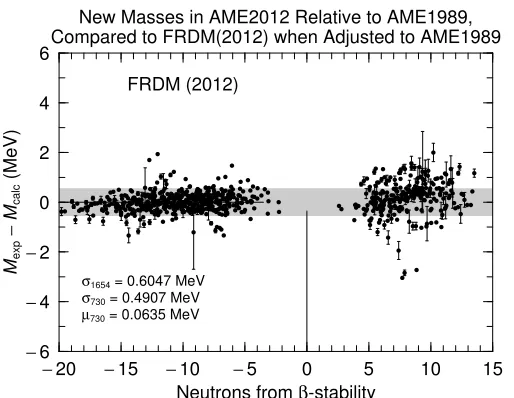
Figure 2.We have adjusted our

current mass model (with all the improvements discussed in [6]) to the older AME1989 experimental evaluation to test the extrapability of the model. It agrees better with the AME1989 data base than

FRDM(1992), due to improvements in the calculations, 0.6047 MeV versus 0.669 MeV for the previous FRDM(1992). But it also extrapolates much better with only 0.4948 MeV deviations for the new nuclei, versus 0.5817 for the previous

FRDM(1992)[8]. From Ref. [6].

3 Single-particle model

Already Bethe and Bacher [2] considered the possibility that microscopic effects might give rise to deviations from the semi-empirical mass model. They noted that in an oscillator single-particle poten-tial there are large gaps in the corresponding single-particle level spectrum and investigated if there were unusually large deviations between their theory and measured masses atZ=20,N=20, namely

40_{Ca. They found none, but concluded that the masses were not measured sufficiently accurately to}

⇐ε2>0.1 ε2<0.1 ⇒

Dubna exp.

Muntian et al. (2003) FRDM (1992) FRLDM (1992) D-Z (1995)

α

-Decay Chain from

117

105 107 109 111 113 115 117

165 167 169 171 173 175 177

Neutron Number

N

Proton Number

Z

7

8

9

10

11

12

Energy Release

Q

(MeV)

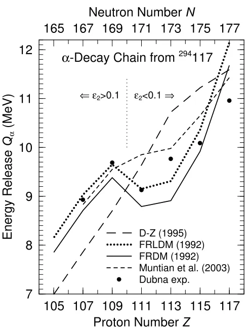
Figure 3.Calculated and measured

Qα-decay energies for294Ts. The

calculated values assume ground-state to ground-state decay, the measured energies may not be, so the differences between measured and calculated values do not directly indicate the degree of (in)accuracy of the underlying mass model. Note that in two of the models the kink observed in the experimental data at Z=107–109 is well reproduced. In this case the kink is related to a change in deformation from spherical to deformed, rather than a gap in the level spectrum at a fixed deformation. D-Z is from Ref. [17] and Muntian from Ref. [18].

4 Strutinsky shell-correction method

⇐ε2>0.1 ε2<0.1 ⇒

Dubna exp.

Muntian et al. (2003) FRDM (1992) FRLDM (1992) D-Z (1995)

α

-Decay Chain from

117

105 107 109 111 113 115 117

165 167 169 171 173 175 177

Neutron Number

N

Proton Number

Z

7

8

9

10

11

12

Energy Release

Q

(MeV)

Figure 3.Calculated and measured

Qα-decay energies for294Ts. The

calculated values assume ground-state to ground-state decay, the measured energies may not be, so the differences between measured and calculated values do not directly indicate the degree of (in)accuracy of the underlying mass model. Note that in two of the models the kink observed in the experimental data at Z=107–109 is well reproduced. In this case the kink is related to a change in deformation from spherical to deformed, rather than a gap in the level spectrum at a fixed deformation. D-Z is from Ref. [17] and Muntian from Ref. [18].

4 Strutinsky shell-correction method

Strutinsky introduced a method that combined physics from the macroscopic liquid-drop model and the single-particle model [15, 16]. Briefly, the potential energy for any prescribed deformation is calculated in the following manner. The energy for the charged liquid drop is calculated for this shape, somewhat simplified it is the sum of a surface and electrostatic Coulomb energy. The single-particle energies are calculated. A shell-plus-pairing correction is then obtained from the calculated single-particle spectrum. In Strutinsky’s method the correction is about−6 MeV when there is a large gap in the spectrum such as in the neutron spectrum atN=126 for208Pb. Since there is also a gap in the proton levels atZ=82 the total shell+plus-pairing correction at spherical shape is about−12 MeV. In situations where there is a high density of levels the shell-plus-pairing correction sum is larger than 10 MeV. We now give some examples of how we have used the macroscopic-microscopic method to provide a multitude of nuclear properties across the nuclear chart. With the continuing increase of computer power over decades it is only during the past 20 or so years this method could be exploited to its full potential.

Calculated Fission-Barrier Height

1 2 3 4 5 6 7 8 Bf(Z,N) (MeV)

130 140 150 160 170 180 190 200 210 220 230 Neutron Number N

80 90 100 110 120 130 Proton Number Z

Figure 4.Calculated fission-barrier

heights for 3282 nuclei. The highly variable structure is mostly due to ground-state shell effects. Ground-state shell effects are particularly strong in the deformed regions around252

100Fm152,270108Hs162and in the nearly spherical region near the next doubly magic nuclide postulated to be at298

114Fl184. The strongest shell effects in this calculation are slightly offset to the left with respect to this isotope. From Ref. [27].

5 Applications of the macroscopic-microscopic method

The first development in this sequence was the introduction of the folded-Yukawa single-particle potential in 1972 [19]. The treatment of the spin-orbit force contribution to the potential has a decisive impact on its success. In the discovery paper the authors used a spin-orbit strength determined in Ref. [20]. In 1973 PM and S-G Nilsson did an extensive study of the optimum spin-orbit strength in the folded-Yukawa and decided on values that are still used today [21]. The first macroscopic-microscopic mass model based on these ideas and an improved macroscopic finite-range “liquid-drop” model [22] appeared in 1981 [23, 24]. Unfortunately, in hindsight it only included about 4000 nuclei, not sufficient to include all r-process nuclei or all nuclei of future interest in the superheavy region. The argument at the time was that we should not blindly let the code crank out numbers without further test of the reliability of the theory. Once comparisons with various types of experimental data and increased computer power were available a mass table extending from the proton to the neutron drip line was completed [8]. This investigation provided masses based on two different macroscopic models, the finite-range liquid-drop model and the finite-range droplet model. It turned out that the latter significantly improved mass predictions. We also note that the expressions used for the neutron and proton single-particle potential radius and depths were since 1972 [19] based on the droplet model ideas and subsequently found to be very realistic and essential [6]. Further development and improved computer performance led to the current mass model FRDM(2012) [6]. As several other groups have done by now, implementation of the FRDM/FRLDM macroscopic-microscopic model can be done based on the complete specifications and mathematical detail found in Refs [6, 8, 19, 22, 25, 26]. It might be useful to note that in Ref. [19] some misprints in Ref. [25] are enumerated.

With this model we also obtain state multipole moments, or equivalently nuclear ground-state shapes. Special types of rare shapes are axially asymmetric and reflection asymmetric shapes. Calculated occurrences of this type of shapes are discussed in Refs. [28, 29].

For some nuclei the potential-energy function versus shape can have several minima. One example is the fission isomeric states which minima correspond to a nuclear shape elongation with the major and minor axes having a ratio of 2:1. Another situation is when there are two minima: one oblate and one prolate, but none as deformed as the fission isomeric state. This situation is referred to as shape coexistence. We have studied globally shape coexistence in Refs. [31, 32].

param-Asymmetric Symmetric 0.2 0.4 0.6 0.8

Fission-Yield Valley-to-Peak Ratio

90 100 110 120 130 140 150

Neutron Number N

70 80 90

Proton Number

Z

Figure 5.Calculated symmetric-yield

to peak-yield ratios for 987 fissioning systems. Black squares (open in colored regions, filled outside) indicateβ-stable nuclei. We find a

new, contiguous region of asymmetric fission separated from the classical location of asymmetric fission in the actinides by an extended area of symmetric fission. From Ref. [30].

eters were adjusted. To obtain similar insight we have adjusted the parameters of the FRDM(2012) to a more limited mass data set [35] and studied the calculated masses obtained for masses measured subsequently. The agreement with subsequently measured masses is shown in Fig. 2 and shows encouraging predictive capability. Another way to assess the predictive properties is to compare do superheavy element (SHE) properties. Some of their properties are obtained through theirα-decay

chains. In Fig. 3 we show a comparison of the FRDM(1992) predictions to more recently observed [36]α-decayQvalues of the decay of294Ts. It is clear the predictions well reproduce the observed interesting structure in the decay chain.

In fission, as we remarked above, the nucleus evolves from a single (ground-state) shape to two separated fission fragments. This process can be studied in the macroscopic-microscopic model by studying the energy of nuclear shapes involved in the transition between the ground state and sepa-rated fragments. A study of a few selected shapes (the only possibility at that time with the limited computer power) showed a definite signature of asymmetric fission for actinides but symmetric fis-sion for somewhat lighter nuclei [37, 38]. It was much later that the macroscopic-microscopic method could be exploited by calculating the potential energy between the ground state and separated frag-ments for the selection of shapes that should be considered, namely elongation, neck radius, left and right fragment spheroidal deformation, and mass split between the fragments [39]. A poorly appreci-ated aspect in this type of calculations is: what is required to identify correctly fission saddle points? A more in-depth account of these aspects is in Ref. [40]. Calculated fission barrier-heights based on these methods are in Ref. [27]. We show in Fig. 4 3282 barrier heights calculated in this approach.

For many simulation applications it is of interest to have available the fission-fragment mass distri-butions. Recently we showed that a Brownian shape motion on calculated five-dimensional potential-energy surfaces well reproduced the observed fission-fragment mass distributions [41–43].

Encouraged by these studies which showed very good agreement with experimental fission frag-ment mass distributions, we went ahead, as we usually do, and made some predictions, so that our model could be tested, of fission fragment mass distributions for an extended region of 987 heavy nuclei [30]. We found a new contiguous region of nuclei predicted to undergo asymmetric fission, see Fig. 5. An earlier “discovery” experiment [44] (which motivated our study) had shown that180_Hg

fissioning asymmetrically inβ-delayed fission. There are still only scattered experiments of fragment

Asymmetric Symmetric 0.2 0.4 0.6 0.8

Fission-Yield Valley-to-Peak Ratio

90 100 110 120 130 140 150

Neutron Number N

70 80 90

Proton Number

Z

Figure 5.Calculated symmetric-yield

to peak-yield ratios for 987 fissioning systems. Black squares (open in colored regions, filled outside) indicateβ-stable nuclei. We find a

new, contiguous region of asymmetric fission separated from the classical location of asymmetric fission in the actinides by an extended area of symmetric fission. From Ref. [30].

eters were adjusted. To obtain similar insight we have adjusted the parameters of the FRDM(2012) to a more limited mass data set [35] and studied the calculated masses obtained for masses measured subsequently. The agreement with subsequently measured masses is shown in Fig. 2 and shows encouraging predictive capability. Another way to assess the predictive properties is to compare do superheavy element (SHE) properties. Some of their properties are obtained through theirα-decay

chains. In Fig. 3 we show a comparison of the FRDM(1992) predictions to more recently observed [36]α-decayQvalues of the decay of294Ts. It is clear the predictions well reproduce the observed interesting structure in the decay chain.

In fission, as we remarked above, the nucleus evolves from a single (ground-state) shape to two separated fission fragments. This process can be studied in the macroscopic-microscopic model by studying the energy of nuclear shapes involved in the transition between the ground state and sepa-rated fragments. A study of a few selected shapes (the only possibility at that time with the limited computer power) showed a definite signature of asymmetric fission for actinides but symmetric fis-sion for somewhat lighter nuclei [37, 38]. It was much later that the macroscopic-microscopic method could be exploited by calculating the potential energy between the ground state and separated frag-ments for the selection of shapes that should be considered, namely elongation, neck radius, left and right fragment spheroidal deformation, and mass split between the fragments [39]. A poorly appreci-ated aspect in this type of calculations is: what is required to identify correctly fission saddle points? A more in-depth account of these aspects is in Ref. [40]. Calculated fission barrier-heights based on these methods are in Ref. [27]. We show in Fig. 4 3282 barrier heights calculated in this approach.

For many simulation applications it is of interest to have available the fission-fragment mass distri-butions. Recently we showed that a Brownian shape motion on calculated five-dimensional potential-energy surfaces well reproduced the observed fission-fragment mass distributions [41–43].

Encouraged by these studies which showed very good agreement with experimental fission frag-ment mass distributions, we went ahead, as we usually do, and made some predictions, so that our model could be tested, of fission fragment mass distributions for an extended region of 987 heavy nuclei [30]. We found a new contiguous region of nuclei predicted to undergo asymmetric fission, see Fig. 5. An earlier “discovery” experiment [44] (which motivated our study) had shown that180_Hg

fissioning asymmetrically inβ-delayed fission. There are still only scattered experiments of fragment

distributions in this region, mainly in the transition regions between symmetric and asymmetric fis-sion, so the predictions still await serious experimental studies. Currently in progress are calculations of fission yields of r-process nuclei for use in r-process fission recycling modeling.

exp. @6.54 MeV

th. based on full Y(Z,N), damp.

50k Tracks ∆ = 1.0 MeV

E*_{=6.54 MeV}

240

Pu

30 40 50 60

Fragment Charge Number Zf

0 5 10 15 20 25

Charge Yield

Y

(

Zf

) (%)

Figure 6.Calculated fission-fragment

charge yields in thermal

neutron-induced fission of239_{Pu. The} calculated yield is based on a calculation ofY(Z,N) in a recent extension of the Brownian shape-motion model [45] which is then summed over neutron number.

Recently we have generalized the Brownian shape-motion model so that we now model the fission-fragment yieldsY(Z,N). The modification is not so much in the Brownian shape-motion model but rather in devising a method to calculate the potential energy of the fissioning nucleus for differentZ/N ratios in the two emerging fragments. This leads to two shape asymmetry variables one inZand one inN. The method and benchmarks are presented in Ref. [45]. In Fig. 6 we compare calculated and experimental charge distributions of240_{Pu. To obtain the charge distribution we summed for eachZ}

the calculatedY(Z,N) over neutron numberN.

Another substantial modeling effort has been and is to calculateβ-decay properties, specifically

decay half-lives and delayed neutron-emission probabilities. Our first global results are in Ref. [33]. A next generation, improved calculation and release will be available in the first half of 2018. PM maintains a web page with publications, figures appearing in these publications and interactive features atURL: http://t2.lanl.gov/nis/molleretal/.

References

[1] C. F. von Weizäcker, Z. Phys.96(1935) 431

[2] H. A. Bethe and R. F. Bacher, Rev. Mod. Phys.8(1936) 82

[3] O. Hahn and F. Strassmann, Naturwiss.27(1939) 11

[4] L. Meitner and O. R. Frisch, Nature143(1939) 239

[5] O. R. Frisch, Nature143(1939) 276

[6] P. Möller, A. J. Sierk, T. Ichikawa, and H. Sagawa, Atomic Data and Nuclear DataTables

109–110(2016) 1

[7] N. Bohr and J. A. Wheeler, Phys. Rev.56(1939) 426

[8] P. Möller, J. R. Nix, W. D. Myers, and W. J. Swiatecki, AtomicDataNucl. DataTables59

(1995) 185

[9] M. Wang, G. Audi, A. H. Wapstra, F. G. Kondev, M. MacCormick, X. Xu, and B. Pfeiffer, Chin. Phys.C36(2012) 1603

[10] M. Mayer, Phys. Rev.75(1949) 1969

[12] M. Mayer, Phys. Rev.78(1949) 22

[13] S. G. Nilsson, Kgl. Danske Videnskab. Selskab. Mat.-Fys. Medd.29:No. 16 (1955)

[14] B. R. Mottelson and S. G. Nilsson, Kgl. Danske Videnskab. Selskab. Mat.-Fys. Skr. .1:No. 8

(1959)

[15] V. M. Strutinsky, Nucl. Phys.A95(1967) 420

[16] V. M. Strutinsky, Nucl. Phys.A122(1968) 1

[17] J. Duflo and A. P. Zuker, Phys. Rev. C52(1995) R23

[18] I. Muntian, Z. Patyk, and A. Sobiczewski, Physics of Atomic Nuclei,66(2003) 1015

[19] M. Bolsterli, E. O. Fiset, J. R. Nix, and J. L. Norton, Phys. Rev. C5(1972) 1050

[20] W. Ogle, S. Wahlborn, R. Piepenbring, and S. Fredriksson, Rev. Mod. Phys.43(1971) 424

[21] P. Möller and J. R. Nix, Proc. Third IAEA Symp. on the physics and chemistry of fission, Rochester, 1973, vol. I (IAEA, Vienna, 1974) p. 103

[22] H. J. Krappe, J. R. Nix, and A. J. Sierk, Phys. Rev. C20(1979) 992

[23] P. Möller and J. R. Nix, Nucl. Phys.A361(1981) 117

[24] P. Möller and J. R. Nix, Atomic Data Nucl. Data Tables26(1981) 165

[25] J. Damgaard, H. C. Pauli, V. V. Pashkevich, and V. M. Strutinsky, Nucl. Phys.A135(1969) 432

[26] K. T. R. Davies, A. J. Sierk, and J. R. Nix, Phys. Rev. C13(1976) 2385

[27] P. Möller, A. J. Sierk, T. Ichikawa, A. Iwamoto, and M. Mumpower, Phys. Rev. C91(2015)

024310

[28] P. Möller, R. Bengtsson, B. G. Carlsson, P. Olivius, and T. Ichikawa, Phys. Rev. Lett.97(2006)

162502

[29] P. Möller, R. Bengtsson, B. G. Carlsson, P. Olivius, T. Ichikawa, H. Sagawa, and A. Iwamoto AtomicData andNuclearDataTables94(2008) 758

[30] P. Möller and J. Randrup, Phys. Rev. C91(2015) 044316

[31] P. Möller, A. J. Sierk, R. Bengtsson, H. Sagawa, and T. Ichikawa, Phys. Rev. Lett.103(2009)

212501

[32] P. Möller, A. J. Sierk, R. Bengtssson, H. Sagawa, and T. Ichikawa, AtomicData andNuclear

DataTables,98(2012) 149

[33] P. Möller, J. R. Nix, and K.-L. Kratz, AtomicDataNucl. DataTables66(1997) 131

[34] P. Möller, R. Bengtsson, K.-L. Kratz, and H. Sagawa, Proc. International Conference on Nuclear Data and Technology, April 22–27, 2007, Nice, France, (EDP Sciences, (2008) p. 69, ISBN 978-2-7598-0090-2), and http://t2.lanl.gov/nis/molleretal/publications/nd2007.html

[35] G. Audi, Midstream atomic mass evaluation, private communication (1989), with four revisions [36] Yu. Ts. Oganessian, J. Phys. G: Nucl. Part. Phys.34(2007) R165

[37] P. Möller and S. G. Nilsson, Phys. Lett.31B(1970) 283

[38] P. Möller, Nucl. Phys.A192(1972) 529

[39] P. Möller, D. G. Madland, A. J. Sierk, and A. Iwamoto, Nature409(2001) 785

[40] P. Möller, A. J. Sierk, T. Ichikawa, A. Iwamoto, R. Bengtsson, H. Uhrenholt, and S. Åberg, Phys. Rev. C79(2009) 064304

[41] J. Randrup and P. Möller, Phys. Rev. Lett.106(2011) 132503

[42] J. Randrup, P. Möller, and A. J. Sierk, Phys. Rev. C84(2011) 034613

[43] J. Randrup and P. Möller, Phys. Rev. C88(2013) 064606

[44] A.N. Andreyev, J. Elseviers, M. Huyse, P. Van Duppen, S. Antalic, A. Barzakh, N. Bree, T.E. Cocolios, V.F. Comas, J. Diriken et al., Phys. Rev. Lett.105, 252502 (2010)