Review Article Open Access
Structure of Single Particles from Randomly Oriented
Ensembles Using an X-Ray Free Electron Laser
SS Kim, S Wibowo and DK Saldin*
Department of Physics, University of Wisconsin-Milwaukee, USA Received: December 01, 2017; Published: December 07, 2017
*Corresponding author:DK Saldin, Department of Physics, University of Wisconsin-Milwaukee, P.O. Box 413, Milwaukee, Wisconsin 53201, USA, Email:
ISSN: 2574-1241
Biomed J Sci & Tech Res
Introduction
As evidenced by the Krebs (or citric acid) cycle [1] life functions via a series of chemical reactions. The experimental study of such reactions is therefore of great interest. Methods of studying such reactions date back at least to fem to second time-resolved photoelectron spectroscopy [2]. High spatial resolution was added by the use of x-rays in the technique of time-resolved crystallography [3]. This latter method originates in the era where there existed only weak X-ray sources. At that time X-rays were used to obtain information about a single molecule only by scattering off a large number of identically oriented copies. Luckily there exist natural structures (crystals) that many substances form which allow this. A typical crystal used in such work contains perhaps a trillion (1012) identically oriented molecules. A problem is that
most chemical reactions in nature do not take place in crystals. Indeed steric hindrance may prevent many important reactions in solution from ever happening in crystals [4].
Two recent developments may allow this limitation to be overcome. One is the development of a much brighter X-ray source
known as a X-ray free electron laser (XFEL). The world’s first
XFEL, the Linac Coherent X-ray Source (LCLS) is now operational at Stanford in the U.S. Another such machine is now operational near Osaka in Japan. Others are planned, in many countries, e.g. Germany, Switzerland, Korea and China. It is true that these machines are very expensive and require the resources of a rich nation or group of nations. Consequently there is likely, by and large, to be only a single machine per country for the foreseeable future
Abstract
The method of time-resolved crystallography offers a method of studying fast changes in structure during a chemical reaction. However, being a crystallographic method it is restricted to crystal structures. The problem with this is that most chemical reactions under physiological conditions happen in solution and not on molecules which are part of a crystal. The main problem with trying to find chemical reactions in solution is that one needs a powerful source of X-rays which will give a measurable signal even from small numbers of randomly oriented molecules. The newly developed X-ray free electron laser allows this when combined with a novel theoretical technique. Of course we understand one of the strengths of working with crystals is that the signal comes not from one but from trillions of identically oriented unit cells. The fact that the unit cells are identically oriented means that the X-rays do not have to scatter off a single molecule (or unit cell) to give a sensible signal. Since all molecules are identically oriented information about an idealized average molecule may be obtained from scattering by a crystal even though the different photons scatter off different molecules. The problem is that most chemical reactions do not take place in crystals.
Two main developments allow us to overcome this limitation. One is the development of the X-ray free electron laser (XFEL) which is capable of producing X-rays many orders of magnitude brighter than any previous X-ray source. If it is possible to determine the structure of a single particle without the need for crystals we will have achieved our goal. Luckily there has been a corresponding increase in understanding of scattering by disordered arrays. One of the things that has become realized recently is that if one concentrates not on the bare intensities of scattering, but on what are known as their angular correlations these said correlations are characteristic, over most of their range, of the structure but on not of the orientation of the molecules, provided the scattering is from a dilute disordered ensemble. Consequently, the way has been opened for the study of molecules via scattering by ensembles that are not identically oriented. What is more, techniques have further been developed for following fast changes in the structure of such molecules in a pump-probe experiment.
(although a second XFEL is planned for the US). There has also been a corresponding improvement of theoretical understanding of fundamental diffraction theory as it had been realized the angular correlations amongst the scattered intensities are characteristic of the structure of a molecule but not of its orientation.
Chemical bonds tend to make each molecule identical apart from their orientations in a solution and the method of angular correlations is ideal to study such reactions. It is true the molecules are swimming in a sea of solvent molecules, in this case largely disordered water molecules. The effects of scattering by solvent have not been studied a lot, but the case of cryo-EM where the molecules swim in vitreous ice, the effect the vitreous ice, consisting of largely randomly oriented waier molecules, the solvent is found not to contribute much to the correlated scattering, and so can be ignored, except that coming from the solvent which might be about 100 times more prevalent that the solute may give rise to Poisson scattering that might interfere with the measured correlations. However, Poisson noise reduces the greater the intensity. Consequently, the scattering by a much larger solvent is actually advantageous.
One of the greatest experimental challenges with single particle work at an XFEL is the extremely low “hit rates” of about 0.1%. This means about 99.9% the beam hits empty solvent which contains no particle of interest. The ability we describe in this paper of obtaining structural information from ensembles of particles allows us to use a much higher concentration and overcomes the hit rate problem. Our hit rates are essentially 100%”
Theory
Before proceeding further we would like to discuss angular pair correlations that play a central part of our theory. Suppose Aj are the scattered amplitudes from protein j of a set that is illuminated. The total intensity expected to be measured in a coherent instrument like an XFEL is thus
2
( , ) j j( , )
I q φ = ∑ A q φ (1)
=j |Aj(q,)|2 + ∑jkj(q,)Ak(q,) eiq.(R
k-Rj) (2)
=j Ij(q,)+ jk A*j(q,) Ak(q,) eiq.(R
k-Rj) (3)
Here the first summation contained on the incoherent
(intensity) summation over different particles (already considered in [5-13] and [14] while the second summation contains the new (coherent) terms which give rise to interparticle interference. Likewise,
I ( q ,+ ) =jI j ( q ,+ ) +jk A *j( q ,+ ) Ak{(q,+) e-iq’.(Rj-Rk) (4)
Where q’ is the scattering vector corresponding to the point (q,,+) on the detector (in polar coordinates). Here also the
first summation contains the incoherent terms and the second
summation contains the interparticle interference additions. So for
coherent scattering, the pair angular correlation defined by
C2(coherent)(q,q,)=< I(q,)I(q,+) d>DP (5)
Where the expression <…>DP represents an average over the measured diffraction patterns and the I’s in the integrand may be taken from (3) and (4). Thus,
C2(coherent)(q,q,)=C
2(incoherent)(q,q,)+ …
+ <Ij (q,) jk Aj(q,+) A*k( +) eiq’.(R
j-Rk) d
>DP …
+< I_j(q, )jk A*J(q,) AK(q,) d >DP e-iq.(Rj-Rk)
d >DP …
+ < jk A *jk A *j( q ,) Ak( q ,) Aj( q ,+ ) A*k(q,+)ei(q-q’).(R
k-Rj) d>DP (6)
Now in integrating over neither q nor q’ ever become zero unless one considers q=0 or q’=0, which only exist under the beam stop, and are therefore not measured. Thus in practice the 2nd and 3rd terms on the RHS are negligible since they are associated with random phases. On the other hand, the 4th term has an argument of the exponential that can become zero even on the resolution ring, and therefore does not need to be small at the points where the argument becomes zero. Here C2(incoherent) contains only contributions from the first incoherent summations in (3) and (4) in addition to
the newer coherent terms. The 4th term contains double sums in (3) and (4). In the end only the 1st and 4th terms survive, and one may write, to a good approximation
C2(coherent)(q,q,)=C2(incoherent)(q,q,)+<jA*j(q,) Ak(q,)
Aj(q,+) Ak*(q, +)x… …ei(q-q’).(R
k-Rj) d>DP (7)
Where C2(incoherent) contains only contribution from the first
(incoherent) summations in (3) and (4) and the remaining term
contains the specifically interparticle interference effects that
arise from the coherence of the XFEL. Here represents the vector in the direction of increasing. For most values of, the randomness of Rj-Rk makes the phases associated with the
exponential random and thus the difference between the coherent and incoherent expressions become negligible. An exception occurs when approaches zero. Then despite the randomness of Rj -Rk the phases of the exponential terms tend towards zero, which is
clearly not random. It will also be noted that at this point Aj(q,+
) Aj(q,) and Ak(q, ) Ak(q,), and so the integrand of (7) Ij(q,) I_k(q,) which is always positive.
Consequently, C2(coherent) is always greater that C_2(incoherent) Thus,
the coherent peak will always be larger than the incoherent peak, as seen by the red part of the curve and consequently at the equivalent point at =2. For a flat Ewald sphere, Friedel’s Law requires
that the intensity at = be equivalent to that at =0, and
hence Figure 1 (which assumes a flat Ewald sphere) has three
Figure 1: Coherent and incoherent C2 correlations for q’=q found from the diffraction patterns of randomly spaced particles by averaging all the diffraction patterns.
Note the difference between the correlations is only that the coherent patterns have an extra high but narrow peaks at (for a flat Ewald sphere, due to Friedel’s Law),
and 2 (same as 0). Alternatively, if one chooses to plot the correlations for |q-q’| greater than the width 2/L, where L is the lateral coherence length, the coherent and incoherent C2’s will be equivalent throughout the entire range [15]. For a dilute ensemble of randomly oriented particles therefore, over most of the range of our previous assumption that C2 be represented by the incoherent value remains true. Thus,
Bl(q,q)=C2(q,q;)Pl(cos((q)cos(q))+sin((q)) sin(q)cos) d
is still valid to a good approximation for coherent radiation. For
a flat Ewald sphere, one can take (q)=and cos((q)}=0 and sin((q))=1, so, to a good approximation,
Bl(q,q)= C2(q,q;) Pl(cos })d (9)
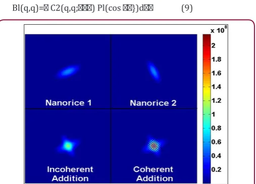
Figure 2: Diffraction patterns of two individual nanorice particles of random orientations (top panels), the diffraction pattern of two incoherently superimposed ones (bottom left panel) and of coherently superposed ones (bottom tight panel).
We next tried to simulate the conditions of a nanoparticles representing a small protein like photoactive yellow protein (PYP)
within a coherence volume that one would expect of a focal spot size
of 0.1 microns (the design specification of the Linac Coherent Light
Source (LCLS) at Stanford, California) and the smallest droplet size claimed of (0.3 microns). This gives an illuminated volume of 0.03 cu. microns. For single particles the resulting diffraction patterns
are as shown on the first two panels of Figure 2, When there are
two randomly oriented particles the diffraction pattern looks like the one in the 3rd column if one assumes no coherence between the two diffraction patterns. When one introduces coherence the diffraction patterns due to two particles appear like that in panel 4, with a set of narrow inference fringes characteristic of the spacing of the particles. Even in this case the values of C2 of the incoherent
and coherent cases are almost identical over most of the range of
due to the randomness of the particle positions making the
specifically coherent terms sum to a small quantity [15] (Figure 2).
Note that only the coherently added diffraction patterns have interference fringes. The effects of the interference fringes on the C2’s almost disappears over most of the range of (q,q;) since the fringes are randomly spaced and oriented. This gives rise to essentially the same C2’s as in the incoherent case except for
isolated regions around at =0, and 2 when the phases become zero and are therefore not random. Similar peaks appear in Kam’s two-point triple correlations C3(q,q;) [10], i.e. they also have narrow peaks at =0, and 2. On the other hand there are no coherent peaks associated with the correlations between different resolution rings such that |q-q’| is greater than 2/L, where L is the transverse coherence length [15].
In this case the integral over the coherent curve in Figure 1 gives almost the same answer as an integral over the incoherent
curve in the same figure that has been considered before, in order to find Bl(q,q). Similarly an integral over C3(q,q;) may be
performed to find a good approximation to Tl(q,q). Since both B and
T are found from the same diffraction pattern (whether it comes from a single particle or several) it is possible to reconstruct an image of a single particle since both C2 and C3 are proportional to the number of particles. Since both C2 and C3 are derived from the
as for single particle, thus allowing exactly the same algorithm for any collection of diffraction patterns corresponding to an arbitrary number of particles. This allows one to reconstruct an image of a single particle from the angular correlations of many, even with the existence of interpartice interference. For incoherent scattering this has been demonstrated in 2D even with experimental data
[6]. However, we think this is the first time this capability has been
demonstrated in 3D (Figure 3).
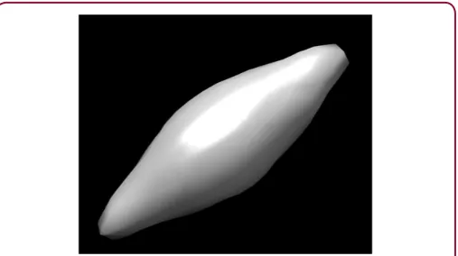
Figure 3: Density of single particle of nanorice of size approximately 50 A recovers from an illuminated area of approximately 1000 A squares from 8000 two particles simulated diffraction patterns including noise and interparticle interference.
In cases where the extra coherent peaks give rise to significant
changes in the values of B, and T, an integral that avoids these points gives almost the same value as the incoherent case. This is a bit like the principal part of an integral in complex analysis, except that the
ordinate is not infinite in this case, the result of the integral over
these regions remains very small. Consequently, the integral over the restricted range for the coherent case gives almost the same result as the integral over the whole range for the incoherent case [15]. It should be noted these deviations between the coherent and
incoherent cases are confined to cases where q=q’ (same resolution
ring). Alternatively, one may avoid this problem if one retrieves information only from different resolution rings (off-diagonal C2’s and C3’s) (or q q’ (since the deviation between the coherent and incoherent cases only occur for the correlations with q=q’ at these localized points). Even if one chooses to obtain information from the terms with q=q’ one may avoid the sharp coherent peaks and obtain the quantity Bl(q,q’) to a good approximation [15].
The B’s can be shown to be essentially
Bl(q,q’)= Nm I*lm(q) Ilm(q) (10)
Where N is the number of particles scattered off. This quantity may contain vital information about the diffraction volume we seek.
Thus, even in the coherent case, one can define
C2(q,q;)= I() I(q,+) d (11)
Where I is the total intensity of the diffraction pattern, provided one avoids the narrow regions around =0 (and their Friedel counterparts) that are characteristic of coherent radiation. At least in 2D it is clear [10] that this is a quantity independent of the orientation of the particle and hence diffraction pattern. (It is in
3D also [7,8]). The quantity depends only on the difference,, the azimuthal angle between two points involved in the calculation of the correlations. Effectively one is comparing the scattering of a single particle in various relative directions, a quantity that is independent of the particle orientation. The fact that this is independent of particle orientation makes it suitable for use with an ensemble of identical particles differing only in orientation. The total signal will be proportional to the number of particles, thus we gain the advantage of a crystal (or at least of a microcrystal) with a signal contributed by multiple particles. Since there are some questions about the feasibility of the signal-to-noise ratio with a large number of particles, the initial tests will be on a small number of particles.
This will be possible since an XFEL will be expected to be initially focused on an area of radius 100 nm, perhaps 20 times larger in linear dimensions than a small protein. The Legendre transform of C2, see Eq. (9), gives rise to a quantity that can be shown to be characterized by the spherical harmonic expansion of the scattered
intensities. That is, it can be shown that if the coefficients I_lm(q) may be extracted from these quantities, one may reconstruct a 3D diffraction pattern of the scattered intensities via the expansion
I(q)=lm Ilm(q) Ylm(,) (12)
Where Ylm(,) is a spherical harmonic of angular momentum quantum numbers (lm). and are 3D polar angles. A problem
is that, in general, the extraction of the Ilm coefficients from the Bl’s is not a trivial task, although there are specific high-symmetry
circumstances when this has been shown to be possible [11,12]. One of these is when there is azimuthal symmetry in the particle for example a grain of nanorice. In this case the azimuthal symmetry of the particle results in an azimuthal symmetry of the diffraction volume [15] If the diffraction volume is azimthally symmetric, one may take m=0 in (10). This immediately suggests
|Il0(q)|=Bl(q,q) (13) This gives the magnitudes of all allowed values of the expansion
coefficients. The only remaining task is to find their phases. They may be found from the diagonal triple correlations defined by
C3(q,q; )=< I2(q,) I(q,+) d>DP (14)
Which may be evaluated from the ensemble of diffraction patterns just as easily as the pair correlations (we don’t need to be concerned about the coherent peak as it is so narrow that we can ignore it His still allows us to capture the incoherent peak Alternatively one can devise an algorithm that uses only C2(q,q’;) with |q’-q|>2/L where L is the width if the illuminated area. It may be shown that over most of the range of
even for coherent radiation (once again it would be best to avoid the red high-intensity peaks in Figure 1 at =0, , and 2 if q=q’ (correlations taken over the same resolution ring) [16].
Reconstruction of a Single Particle from Multiple Particle
Diffraction Patterns
for by the XFEL instrument manufacturers and the sizes of typical proteins. Suppose one uses a concentration of 0.6 moles/ m3 as in SAXS. The design specification of the world’s first X-ray free electron
laser (XFEL), the Linac Coherent Light Source (LCLS), is for a focal spot size is about 0.1 micron square, and since the minimum size of a liquid droplet claimed is about 0.3 microns [17], the volume illuminated will be about 3x10-21m3, or else about 1.8x10⁻²¹ moles.
But Avogadro’s number is about 6x10 molecules/mole. Thus the minimum number of molecules illuminated will be about would be about 400.
Thus we have to conclude that for the study of small proteins such as PYP, single molecule studies are still some way in the future, and that, in the meanwhile, we need either nanocrystals or a number of independently randomly oriented molecules, and a theory of type presented here if clustering of the molecules can be avoided. If the molecules cluster, it’s probably better to use a
“hit-finder” to eliminate multiple particle hits beforehand and then to
use any of the theories proposed (including this one) for structure solution
Although this has been claimed before [7,8], we have now actually tested this proposition in real simulations, not stopping at showing that the correlations are the same (apart from a scaling factor), but reconstructing an image from two particles per shot from the correlations. We have shown that a particle may be reconstructed from both Bl(q,q) and Tl(q,q)’s from a single particle if m=0. We show here that exactly the same method may be used for multiple particles in independent random orientations in each snapshot diffraction pattern since the scaling factor of both B and T are the same for a given number of particles. This will always be the case: the diffraction patterns from which B and T are evaluated will come from exactly the same numbers of particles since in general they will be from the same diffraction patterns. For purposes of illustration here we considered only two particles in independent random orientations, but this illustrates the main point. We simulated
I’lm(q) = m.[Dlm,m’(1,1, 1)+Dlm,m’(2, 2, 2) ] Ilm(q) (15)
Where (1, 1, 1) and (2, 2, 2) are independent sets of random Euler angles. We did explicit simulations of the expected diffraction patterns and calculated from them the angular correlations B and T and reconstructed from them, by the same algorithm for the single-particle case, a real space image. The image we found is shown in Figure 3.If indeed the conditions of a dilute ensemble of identical particles can be achieved, there will
be no need for a hit-finder program [18] to reject multiple-particle
hits provided the particles are truly random in position (dilute ensemble). The fact that the particle-number-dependent scaling factors are the same for the pair and two-point triple correlations means it is not necessary to know at the outset exactly how many particles there are in the ensemble since both the pair correlation and two-point triple correlations are derived from diffraction patterns with exactly the same number of particles.
The possibility of using diffraction patterns possibly from multiple particles adds considerably to the capability of the use for
the XFEL for structure determination of individual particles as it will add greatly to the “hit-rate”. Our simulations suggest that here may be even advantages to considering diffraction patterns from ensembles of multiples in terms of convergence. In light of this the
only case we see for hit-finder program at least one that determines
single particle hits is when the particles tend to stick together and agglomorate. In such a case it might be better to determine the structure from single particles. In should be pointed out that despite the fact that it is capable of dealing with cases of multiple randomly oriented particles, it is also a method of determining the structure of a single particle from diffraction patterns of a single particle in random orientations [18].
The values the magnitudes of the spherical harmonic expansion
coefficients are determined from (13). Also, as Bl(q,q) is determined by the integral of a real quantity C2 with a real Legendre polynomial, it is real and has a positive square root. The only remaining task is to determine the sign of Il0(q). We can determine this sign from the triple correlations by assuming, as it must be for nanorice,that azimuthal symmetry of the amplitudes implies azimuthal symmetry of the intensities from the usual Clebsch-Gordon rules for adding angular momenta. In this case, all magnetic quantum numbers are equal to zero, and the triple correlation reduces to a sum over only the angular momentum quantum numbers l, and not also magnetic quantum numbers m. Thus,
Tl(q,q)=N∑ Il0(q) I0(q)l0 (q) G(l0; 0; 0) (16)
Where G is a gaunt coefficient [19] Note that the two-point
triple correlations are scaled for multiple particles by exactly the same factor N as the quantities Bl.
Since an ellipsoid has azimuthal symmetry about a particular axis, we can choose that particular axis as z-axis, thus eliminating any other components of the magnetic quantum number except m=0. |Il0(q)| can be obtained directly from Bl(q,q) via (13). The only unknown here is sign of I_{l0}(q). The sign can be determined
by fitting all possible signs of Il0(q) to the values Tl(q) of the triple correlations calculated directly from the diffraction patterns of random particle orientations in (16). It should be stressed that the number of equations is equal to the number of distinct Tl(q,q) values, namely the numbers of q and l values, as is the number of unknowns Il0(q), so there is no information deficit [20] (Figure 3).
After obtaining the signs of the Il0(q), the single particle diffraction volume can be calculated from
I(q)=∑l Il0(q) Yl0(q) (17)
And an iterative phasing algorithm produces the real space image of Figure 3.
3 was obtained from diffraction pattern intensities simulated under the coherence assumption since the difference between the coherent and incoherent intensities are highly localized at =0,
π and 2π in the angular correlations.
Experimental Determination of the Time-Resolved
Structure of Proteins
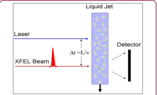
Armed with these facts about angular correlations, and their remarkable ability to study structure from disordered ensembles, we return now to the main problem addressed in this paper, namely the recovery of time-resolved information about proteins from XFEL diffraction patterns. Paradoxically, it is easier to extract useful information from more complex particles in a time-resolved experiment of the form of Figure 3, although the advantages suggested above of not needing to focus on a single particle remain. In this arrangement the particles are incident on an XFEL in a liquid jet. A short time before the incidence of the X-ray beam on the liquid jet it is illuminated by light from an optical laser which puts suitable molecules into a light-induced excited state. A schematic diagram of the apparatus is shown in Figure 4. Although this experiment describes excitation by light, other similar experiments may be considered in which one studies the set of molecules immediately after they has been mixed with a substrate, for example. As we have already seen.
Figure 4: Schematic diagram of the experiment on deducing time-resolved structure from disordered ensembles.
A quantity that is independent of the particle’s orientation (although dependent of the particle structure) is those related, example to the angular pair correlations, C2. This will undoubtedly change Bl(q,q’) by a quantity B(q,q’), which in turn may be measured by measuring the values of B. before and after the
reaction. Interestingly, it is possible to find a linear relation
between l(q,q’) and the change in the electron density (r) of the molecule. Since in general there will be a time delay between the optical laser excitation of the molecule and its interrogation by the X-ray beam, if the structure after the excitation may be deduced from the measured X-ray diffraction patterns, one would
get a handle into the structure a specified time after the excitation.
Since this time interval may be varied by just choosing to illuminate the particle beam a different distance from the incidence of the X-ray beam, one is able to follow the time-resolved changes in the
structure of the photo excited molecule that is the course of light-induced chemical reaction.
The central experimental quality one uses is Bl(q,q’) which we have seen is the Legendre transform of C2(q,q’;∆) which, being a pair correlation, is characteristic of the particle structure, but
not of its orientation [7,8]. We ultimately want to find the change
p(r) in the electron density of each molecule (assumed identical, as one must expect of molecules) corresponding to an Bl(q,q’) which in turn is derived from the experimentally measured C2(q,q’;
). It can be shown that the quantity Bl(q,q’) can rewritten in the alternative form
Bl(q,q’)=NmI*lm(q)Ilm(q’) (18) Differentiating which, we obtain
Bl(q,q’)=Nm Ilm(q)Ilm(q’) + Ilm(q)Ilm(q’ ) (19)
In terms of the spherical harmonic expansion coefficients
Ilm(q) of the diffraction volume of a single particle. Also note that
Ilm(q) = I(q) Ylm(q) dq. (20)
In order to relate this to the change in the electron density one should convert small changes in the intensity to small changes
A in the amplitude, which one can do by differentiating. Since I(q)=|A(q)|^2 (21) It follows taking the variation again that
I(q)=A(q)*A(q)+A*(q)A(q) (22)
At first sight it is a bit disappointing that both A and its complex conjugate appear on the RHS. However as we will see, this is of little consequence since the quantity we are ultimately after, namely the change in the electron density of the molecule, (r), is real. Since
A(q)= (r})ei q.r dr (23) And the complex conjugate of this equation is
A*( q)=( r)) e-i q.r dr (24)
It’s possible to relate both to the change (r) in the real
electron density. In summary, it is possible to find a linear real
relation
Bl(q,q’)=N Mlqq’;j(rj) (25) Where Mlqq’,j=lmI*lm(q) Clm(q’,rj)+C*lm(q,rj) Ilm(q’) (26) Where Clm(q,rj)=eiq.rj4klmfk il jl(q|rk-rj|)Y*lm(|rk -rj|) (27)
unexcited molecule. They both recover the difference density
in the frame of reference of the “dark” structure. In both cases, the latter factor allows the difference electron density to be displayed ultimately using standard crystallographic software superimposed on a model of the “dark” structure that the changes in the structure on photoexcitation are more obvious. It should be noted that although individual particles are in random orientations an initial reconstruction of the angular correlations allows one to reconstruct the electron density in an orientation of one choosing (since all orientations correspond to the same angular correlations). We choose the frame of reference of the “dark” structure, by a suitable
definition of the matrix M, because it allows the display of the
electron density changes using exactly the same software as time-resolved work with crystals.
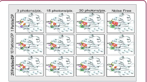
One thing we should point out is that like the difference Fourier method, this is a non-iterative way of getting at the difference electron density directly from the measured data. It seems to be accurate enough to determine structural changes at the level of the residues of a protein. This is seen in Figure 5 [22] in which is shown the expected difference electron density calculated by our algorithm of the expected difference structure of photoactive yellow
protein (PYP) 2 ms after photoexcitation. This figure suggests that
the reconstruction survives Poisson noise which is included in the simulations. It will be noted that after 2ms two residues are expected to move simultaneously, the chromophore as well as the nearby ARG residue which moves in response. Some evidence of the movement of both is just seen in the reconstructions, although the larger movement of the chromophore is more evident. As is customary in time-resolved work, the red regions indicate a
deficiency of electron density in the final image and a green lobe
indicates an increase in the electron density. Thus looking at these electron density maps gives an indication of the structural changes a short time measured time after photoexcitation.
Figure 5: Difference electron density expected 2ms after photoexcitation. These calculations offer a realistic simulation as they assume that the diffraction patterns include Poisson noise. We consider three different numbers of particles as well as three different incident photon counts.
In keeping with our featured capability of the correlation method it will be noted that the right hand column features as many as 25 randomly oriented particles. These simulations were performed assuming an incoherent source of X-rays as the intensity
from many particles is assumed to be the sum of intensities from single particles. The distinction with the coherent case is not very important over most of the range of the correlations as the randomness of particle positions give the scattering a kind of incoherence [9]. The only region where the coherence plays a part in when q=q’ and is approximately zero, (due to Friedel symmetry) or 2 (same as zero). We have suggested how to deal with these differences [15] (Figure 5)
Conclusion
The significance of this work is that if these simulations are realized in practice, we now have, for the first time, a method of finding the structures of particles such as molecules from diffraction
patterns of copies of many of the molecules even if they are not of identical orientations as in a crystal. In the last application we have shown that even time-resolved structure may be determined of molecules that are in random orientations, thus opening to experimentally observing realistic chemical reactions. It should be pointed out that many of the effects we have ignored, such as scattering by solvent, are fairly unimportant for the time-resolved problem since here we look at differences in the correlations between the photo excited and ground state molecules, where such factors tend to subtract out. Indeed in the time-resolved problem we study only features of the diffraction patterns that are different due to the photoexcitation. Of course solvent is perhaps 100 times as prevalent as solute and could give rise to Poisson noise that does not cancel between the photo excited and ground state structures so some care has to be exercised.
An experiment has recently been reported in which the structure of the Mimi virus has been determined experimentally by a variant of the single particle methods described earlier [23]. It has been previously shown by us [10,11] that under various high-symmetry situations, that it is possible to determine the structure of the particle from simulated diffraction patterns. In an experiment to recover time-resolved structural variations, starting from a knowledge of a nearby structure, using many of the same quantities, namely, the angular correlations, have also been shown to be capable of recovering time-resolved changes in a structure from the knowledge of a closely related structure of a single molecule in realistic simulations, including shot noise [24] even from diffraction patterns of multiple particles, as we demonstrate here. This possibility is unprecedented in structural work with XFEL diffraction patterns. This method also works on diffraction patterns of multiple particles in independent random orientations.
Acknowledgment
We acknowledge support for this work from the National Science Foundation, grant numbers MCB-1158138 and STC-1231306, we thank Kanupriya Pande, Ruslan Kurta, Peter Zwart and Jeffery Donatelli, for helpful discussions, and Kanupriya Pande for comments on the manuscript.
References
2. A Stolow, AE Bragg, DM Neumark (2004) Femosecond Time-Resolved Photoelectron Spectrioscopy. Chem Rev 104(4): 1719-1757.
3. K Moffat, D Szebenyi, D Bilderback (1984) X-ray Laue diffraction from protein crystals. Science 222(4645): 1423-1425.
4. TW Kim, JH Lee, J Choi, KH Kim, LJ van Wilderen, et al. (2012) Protein structural dynamics of photoactive yellow protein in solution revealed by pump-probe X-ray solution scattering. J Am Chem Soc 134(6): 3145-3153.
5. DK Saldin, VL Shneerson, M Howells, S Marchesini, HN Chapman, et al. (2010) Structure of a single particle from scattering by many particles randomly oriented about an axis: towards structure solution without crystallization. New J Physics 12: 035014.
6. DK Saldin, HC Poon, M Bogan, S Marchesini, D Shapiro, et al. (2011) new light on disordered ensembles: ab initio structure determination of one particle from scattering fluctuations of many copies. Phys Rev Lett 106(11): 115501.
7. Z Kam (1978) Determination of macromolecule structure in solution by spatial correlations. Macromolecules 10: 927.
8. DK Saldin, VL Shneerson, R Fung, A Ourmazd (2009) Structure of isolated biomolecules from ultra-short x-ray pulses: exploiting the symmetry of random orientation. J Phys Condens Matter 21(13): 134014.
9. DK Saldin, HC Poon, VL Shneerson, M Howells, HN Chapman, et al. (2010) beyond small angle X-ray scattering: exploiting angular correlations. Phys Rev B81: 174105.
10. HC Poon, DK Saldin (2011) beyond the crystallization paradigm: structure determination from diffraction patterns of ensembles of randomly oriented particles. Ultramicroscopy 111(7): 788-806. 11. DK Saldin, HC Poon, P Schwander, M Uddin, M Schmidt (2011)
Reconstructing an icosahedral virus from single particle diffraction experiments. Opt Exp 19(18): 17318-17335.
12. HC Poon, P Schwander, M Uddin, DK Saldin (2013) Fiber diffraction without fibers. Phys Rev Lett 110(26): 265505.
13. R Kirian, KE Schmidt, X Wang, RB Doak, JCH Spence (2011) Signal, noise, and resolution in correlated fluctuations from snapshot small angle x-ray scattering. Phys Rev 84(1): 011921.
14. DK Saldin, HC Poon, VL Shneerson, M Howells, HN Chapman, et al (2010) beyond small angle X-ray scattering: exploiting angular correlations. Phys Rev B 81: 174105.
15. RP Kurta, M Altarelli, E Weckert, IA Vartnyants (2012) X-ray cross correlation analysis applied to disordered two dimensional systems. Phys Rev B85: 184204.
16. We have earlier considered another case where the diffraction volume is dominated by m=0. This is the case of a helical structure, which is also characterized by intensities only on a set of ``layer planes’’. In the present case the azimuthally symmetric diffraction volume is not characterized by ``layer planes’’. The fact that the intensities appear throughout reciprocal space provides the distinction.
17. DP Deponte, JT McKeown, U Weirstall, RB Doak, JCH Spence (2011) Towards ETEM serial crystallography: electron diffraction from liquid jets. Ultramicrosc 111(7): 824-827.
18. JB Pendry (1974) it Low Energy Electron Diffraction. Academic, London, UK.
19. V Elser (2011) Strategies for processing diffraction patterns from randomly oriented particles. Ultramicrosc p. 111.
20. ND Loh, MJ Bogan, V Elser, A Barty, S Boutet, et al. (2010) Cryptotomography: reconstructing 3D Fourier intensities from randomly oriented single-shot diffraction patterns. Phys Rev Lett 104: 225501.
21. K Pande, P Schwander, M Schmidt, DK Saldin (2014) Deducing fast electron density changes in randomly oriented uncrystallized biomolecules in a pump-probe experiment. Phil Trans Roy Soc B 369(1647): 20130332.
22. K Pande, M Schmidt, P Schwander, DK Saldin (2015) Simulations on time-resolved structure determination of uncrystallized biomolecules in the presence of shot noise. Struct Dyn 2(2): 024103.
23. J Drenth (2007) Principles of Protein X-Ray Cryatsllography Berlin: Springer.
24. T Ekeberg, M Svenda, C Abergel, FR NC Maia, V Seltzer JM Claverie, et al. (2015) The dimensional reconstruction of the giant mimivirus particle with an x-ray free electron laser. Phys Rev Lett 114: 098102.
Assets of Publishing with us • Global archiving of articles
• Immediate, unrestricted online access • Rigorous Peer Review Process • Authors Retain Copyrights • Unique DOI for all articles