Fuzzy
H
∞Output Feedback Control of Nonlinear
Systems Under Sampled Measurements
Sing Kiong Nguang
∗Department of Electrical and Electronic Engineering,
The University of Auckland, Private Bag 92019 Auckland, New Zealand.
Email: [email protected]. Fax: (+64 9) 3737461
Peng Shi
Land Operations Division, Defence Science & Technology Organisation,
PO Box 1500, Salisbury SA 5108, Australia.
Email: [email protected]. Fax: (+61 8) 82595055
Abstract
This paper studies the problem of designing an H∞ fuzzy feedback control for a class of nonlinear systems. A nonlinear systems is first described by a continuous-time fuzzy system model under sampled output measurements. The premise variables of the fuzzy system model are allowed to be unavailable. We develop a technique for designing an H∞ fuzzy feedback control which globally stabilises this class of fuzzy system models. A design algorithm for constructing the H∞ fuzzy feedback controller is given. A numerical simulation example is given to show the potential of the proposed techniques.
Keywords: Fuzzy systems, sampled measurements, H∞ control, Output feedback.
1
Introduction
There has been some substantial interest over the past few years in the direct design of digital controllers using continuous-time performance measures. One of the interesting approaches is the hybrid optimalH∞control approach. So far a number of different techniques have been
proposed to provide solutions to the hybrid optimal H∞ control problems. The techniques include: 1) lifting technique [1, 2, 3, 4] which consists of transforming the original sampled-data system into an equivalent LTI discrete-time system with infinite-dimensional input-output signal space. Then L2 induced norm of the sampled-data system is shown to be less
than one if and only if the H∞ norm of this equivalent discrete system is less than one; 2) descriptor system technique [5] where the system is first represented by a hybrid state space model and the solution to theH∞sampled-data problem is then characterised by the solution of certain associated Hamilton-Jacobi equation; 3) technique based on linear systems with jumps [6]-[17] which is a direct characterisation of the problem in the similar terms to those of standard LTI H∞ control problems, and leads to a pair of Riccati equations. Recently, linear H∞ sampled-data results have been extended to nonlinear systems under sampled
measurement. In [18]-[22], solutions to the nonlinear H∞ sampled-data control problem have been obtained in terms Hamilton-Jacobi equation (HJE). However, until now, it is still very difficult to solve for a global solution to the Hamilton-Jacobi equation (HJE).
To design a model-based controller for a given process, a mathematical model which captures all the relevant characteristics of the process is required. Many practical systems are very complex, a suitable mathematical model that describes the dynamics of processes is very difficult, if not impossible to obtain. However, many of these systems can be expressed in some form of mathematical model locally or as an aggregation of a set of mathematical models. Based on this idea, Takagi, Sugeno and Kang have proposed a fuzzy inference system known as the TSK model in fuzzy system literature. For the representative work on this topic, we refer readers to the papers of [23]-[32]. This modelling approach provides a powerful tool for modelling complex nonlinear systems. Unlike conventional modelling where a single model is used to describe the gloabl behavior of a systems, TSK modelling is essentially a multimodel approach in which simple submodels (typically linear models) are combined to describe the global behavior of the system.
Typically, a continuous-time Takagi-Sugeno fuzzy dynamic model is locally described by a set of linear models and is represented by fuzzy IF-THEN rules that have the form
Plant Rule i:
˙
x(t) =Aix(t) +Biu(t), i= 1,2,· · ·, r
where ν1(t),· · ·, νϑ(t) are the premise variables, Mij(j = 1,2,· · ·, ϑ) are fuzzy sets that are
characterised by membership functions, x(t)∈ <nis the state vector, u(t)∈ <m is the input, the matrices Ai andBi are of appropriate dimensions andris the number of IF-THEN rules.
Given a pair [x(t)u(t)], by using a singleton fuzzifer, product fuzzy inference and weighted average defuzzifier, the final state of the fuzzy system is inferred as follows:
˙
x(t) =
Pr
i=1JPi(ν(t))[Aix(t)+Biu(t)]
r
i=1Ji(x(t))
= Pri=1µi(ν(t))[Aix(t) +Biu(t)]
(1.1)
where Ji(ν(t)) is the weight of each rule and it is calculated as follows:
Ji(ν(t)) =
ϑ
Y
j=1
Mij(νj(t)), µi(ν(t)) =
Ji(ν(t))
Pr
i=jJj(ν(t))
Mij(νj(t)) is the grade of membership of νj(t) in Mij. It is assumed in this paper that
Ji(ν(t))≥0, i= 1,2,· · ·, r; r
X
i=1
Ji(ν(t))>0
for all t. Therefore
µi(ν(t))≥0, i= 1,2,· · ·, r; r
X
i=1
µi(ν(t)) = 1
for all t. For the convenience of notations, let Ji =Ji(ν(t)) andµi =µi(ν(t)); then the final
state of the fuzzy system can be represented as
˙
x(t) =
r
X
i=1
µiAix(t) +
r
X
i=1
µiBiu(t). (1.2)
For the fuzzy controller design, it is supposed that the fuzzy system is locally controllable. First, the local state feedback controllers are designed as follows, based on the pairs (Ai, Bi):
Controller Rule i:
IF ν1(t) is Mi1 and · · ·and νϑ(t) is Miϑ THEN
then, the final fuzzy controller is
u(t) = −
r
X
i=1
µiKix(t).
In practice, not all the state are available. Indeed, for a continuous-time systems, the output measurement are often available at discrete points, i.e., measured at sampled points. Therefore, it is necesary and practical useful to design an observer to estimate the system state. In [33, 34], by restricting the premise variables (ν1,· · ·, νϑ) to be measurable, a fuzzy
observer has been developed. This restriction enables the authors in [33, 34] to select the fuzzy sets of the fuzzy observer to be the same as the fuzzy sets of the plant. Hence, the development of the separation property of controller and filter is possible. In general, however, the premise variables for a general TSK model can be unavailable. In this case, the premise variables of the fuzzy observer can not be selected to be the same as the premise variables of the plant. Hence, the results given in [33, 34] can not be applied. What we intend in this paper is to design an H∞ output feedback controller by allowing the premise variables of the plant to be unavailable.
Notation. Most of the notations used in this paper are fairly standard. <n and <n×m
denote respectively, thendimensional Euclidean space and the set of alln×mreal matrices. The superscript “t” denotes matrix transposition and the notation X ≥ Y(respectively,
X > Y) whereX and Y are symmetric matrices, means that X−Y is positive semi-definite
(respectively, positive definite). L2[0, T] stands for the space of square integrable vector
functions over [0, T], l2(0, T) is the space of square summable vector sequences over (0, T), k · k[0,T] will refer to the L2[0, T] norm over [0, T] and k · k(0,T) is the l2(0, T) norm over
(0, T). T is allowed to be ∞ and in this case by the notation [0, T] we mean [0,∞). F(θ−) and F(θ+) stand for the left limit and right limit of a function F(θ), respectively.
2
System Description and Definition
The class of nonlinear sampled-data systems under consideration is described by the following fuzzy system model:
Plant Rule i:
IF ν1(t) is Mi1 and · · ·and νϑ(t) is Miϑ THEN, for i= 1,2,· · ·, r:
˙
z(t) = C1x(t), t 6=mh (2.2)
zd(mh) = Cdx(mh), (2.3)
y(mh) = C2ix(mh) +D21v(mh), (2.4)
where Mij(j = 1,2,· · ·, ϑ) are fuzzy sets, x(t) ∈ <n is the state, x0 is an unknown initial
state, w(t)∈ <p is the disturbance input, u(t)∈ <m is control input,y ∈ <` is the sampled measurement, v ∈ <q is the measurement noise, z ∈ <r is the controlled continuous output, zd ∈ <s is the controlled discrete output, 0< h ∈ < is the sampling period, m is a positive
integer, Ai, B1, B2i, C1, C2i, Cd and D21 are known real time-varying bounded matrices of
appropriate dimensions withAi, B1, B2i, C1 andD12being piecewise continuous, andr is the
number of IF-THEN rules.
Throughout this paper, we adopt the following standard H∞ assumptions.
Assumption 2.1
D21[B1t D
t
21] = [0 I]. (2.5)
Assumption 2.2 (eAih, C
2i) are observable and (Ai, B2i) are controllable.
The resulting fuzzy system model is inferred as the weighted average of the local models and has the form
˙
x(t) =
r
X
i=1
µiAix(t) +B1w(t) +
r
X
i=1
µiB2iu(t), t6=mh, x(0) =x0 (2.6)
z(t) = C1x(t), t6=mh (2.7)
zd(mh) = Cdx(mh) (2.8)
y(mh) =
r
X
i=1
µiC2ix(mh) +D21v(mh). (2.9)
We are concerned with designing a fuzzy H∞ output feedback control law G for (2.6)-(2.9), based on the sampled output measurements of (2.9) such that the controller G reduces z uniformly for any wandv in the sense that given a scalar γ >0, the worst-case performance measure of closed-loop system of (2.6)-(2.9) with the controller G, defined by:
Z T
0
zT(t)z(t)dt+
k
X
m=1
zdT(mh)z(mh)≤γ2
(Z T
0
wT(t)w(t)dt+
k
X
m=1
vT(mh)v(mh)
)
(2.10)
The control problem we address in this paper is as follows: Given a scalar γ >0, design a fuzzy controller (G) based on the sampled measurements, y(mh), such that (2.10) holds:
Note that the performance measure in (2.10) is in terms of not only of the controlled signals at the sampling instants but also of the continuous-time controlled output between the sampling instants. This allows the intersampling behaviour to be taken into account in the control design. When only the controlled continuous output is considered, (2.10) will reduce to the performance measure used in [8].
Remark 2.1 It should be remarked that (2.8)-(2.9) can be viewed as a “mixedL2/`2” output
signals. In real environmental systems, we always face continuous-time systems, discrete-time systems, sampled-data systems and hybrid systems, i.e., systems with both continuous-and discrete-time states. The study of this kind of systems is motivated by robust sampled-data control, filtering and loop transfer recovery of sampled-sampled-data systems [14].
In this paper, we consider the following H∞ fuzzy output feedback controller,G:
Controller Rule i:
IF ˆν1(t) is Mi1 and · · ·and ˆνϑ(t) is Miϑ THEN
˙ˆ
x(t) = aixˆ(t) +biu(t), t6=mh
ˆ
x(mh) = xˆ(mh−) +L
i
y(mh)−yˆ(mh)
ˆ
y(t) = C2ixˆ(t)
u(t) = Kixˆ(t)
for i= 1,2,· · ·, r (2.11)
where ˆνi(t) are the premise variables of the controller, ˆx(t)∈ <nis the controller state vector,
ˆ
y(t)∈ <` is the controller output,a
i are the controller matrices,bi are the input matrices,Li
are the observer gains, Ki are the controller gains, and r is the number of IF-THEN rules.
The final H∞ fuzzy output feedback controller is inferred as follows:
˙ˆ
x(t) = Pri=1µˆiaixˆ(t) +Pri=1µˆibiu, t6=mh
ˆ
x(mh+) = xˆ(mh) +Pri=1µˆiLi
y(mh)−yˆ(mh)
ˆ
y(t) = Pri=1µˆiC2ixˆ(t)
u(t) = Pri=1µˆiKixˆ(t).
(2.12)
However, in general, it is extremely difficult to derive an accurate fuzzy systems model by imposing that all the premise variables are measurable. In this paper, we do not impose that condition, we choose the premise variables of the controller to be different from the premise variables of the fuzzy system model of the plant.
Using (2.12), the control problem can be reformulated as follows:
Problem Formulation: Given a scalar γ >0, design an H∞ fuzzy output feedback controller of the form (2.12) such that the inequality (2.10) holds.
In the sequel, without loss of generality, we assume γ = 1. Let us denote the estimation error as
e(t) =x(t)−xˆ(t). (2.13)
By differentiating (2.13), we get
˙
e(t) = x˙(t)−x˙ˆ(t)
=
r
X
i=1
µiAix(t) +B1w(t) +
r
X
i=1
µiB2iu(t)−
r
X
i=1
ˆ
µiaixˆ(t)−
r
X
i=1
ˆ
µibiu(t)
=
r
X
i=1
(µi−µˆi)Aix(t) + r X i=1 r X j=1
(µi−µˆi)ˆµjB2iKj[x(t)−e(t)] + r
X
i=1
ˆ
µiAix(t)
−
r
X
i=1
ˆ
µiai[x(t)−e(t)] +B1w+
r X i=1 r X j=1 ˆ
µiµˆj{B2i−bi}Kj[x(t)−e(t)], t6=mh
=
r
X
i=1
(µi−µˆi)Aix(t) + r X i=1 r X j=1
(µi−µˆi)ˆµjB2iKj[x(t)−e(t)]
+
r
X
i=1
ˆ
µiµˆj
Ai−ai−biKj+B2iKj
x(t) +B1w
+ r X i=1 r X j=1 ˆ
µiµˆj
ai+bi−B2i
Kj[x(t)−e(t)], t6=mh
e(mh+) = e(mh)−
r X i=1 ˆ µi r X i=1 ˆ
µjLi
C2jx(t) +D21v(mh)−C2jxˆ(t)
= e(mh)−
r X i=1 r X j=1 ˆ
µiµˆjLiC2je(mh)−
r X i=1 r X j=1 ˆ
µi(µj −µˆj)LiC2j
x(mh)−e(mh)
+ r X i=1 ˆ
The system (2.6) with (2.12) can be represented as follows:
˙
x(t) = Pri=1
Pr
j=1µˆiµˆj[Ai+B2iKj]x(t)−Pri=1
Pr
j=1µˆiµˆjB2iKje(t)
+Pri=1
Pr
j=1(µi−µˆi)ˆµjB2iKj[x(t)−e(t)]
+Prj=1(µi−µˆi)Aix(t) +B1w(t), t6=mh
x(mh+) = x(mh).
(2.15)
Using (2.14) and (2.15), we get the augmented system of the following form:
˙˜
x(t) =
x˙(t)
˙
e(t)
= Pri=1
Pr
j=1µˆiµˆj
Ai+B2iKj −B2iKj
Ai+B2iKj−ai−biKj ai −B2iKj +biKj
x˜(t)
+Pri=1
Pr
j=1(µi−µˆi)ˆµj
Ai+B2iKj −B2iKj
Ai+B2iKj −B2iKj
x˜(t) +Pri=1µˆi
B1
B1
w(t)
= Pri=1
Pr
j=1µˆiµˆj
Aijx˜(t) + Ψiw(t)
+Prj=1µˆjfj(x(t))˜x(t), t6=mh
(2.16)
˜
x(mh+) = Pr
i=1
Pr
j=1µˆiµˆj
I 0
0 I−LiC2j
x˜(mh)
+Pri=1
Pr
j=1µˆi(µj −µˆj)
0 0
−LiC2j LiC2j
x˜(mh)
+Pri=1µˆi
0
−LiD21
v(mh)
= Pri=1
Pr
j=1µˆiµˆj
( ¯Aij+Hi∆F E)˜x(mh) + Υiv(mh)
(2.17)
where
Aij =
Ai+B2iKj −B2iKj
Ai+B2iKj−ai−biKj ai −B2iKj +biKj
(2.18)
¯
Aij =
I 0
0 I−LiC2j
, Hi =
0
Li
(2.19)
fj(˜x(t)) =
∆A 0 ∆A 0
+
∆BKj −∆BKj
∆BKj −∆BKj
Ψi =
B1
B1
, Υi =
0
−LiD21
, E =
−C21 C21
.. . ...
−C2r C2r
(2.21)
∆F = [(µ1−µˆ1) · · · (µr−µˆr)], ∆B = r
X
i=1
(µi−µˆi)Bi, ∆A= r
X
i=1
(µi−µˆi)Ai. (2.22)
3
Fuzzy Output Feedback Control Design
In this section, we convert the problem ofH∞fuzzy output feedback control to the solvability
of differential Riccati inequalities with jumps.
Theorem 3.1 Given the augmented system (2.16)-(2.17) satisfying Assumptions 2.1 and 2.2, if there exists a positive definite symmetric solution P such that for i, j = 1,2,· · ·, r, the following differential Riccati matrix inequalities with jumps hold:
˙
P(t) +ATijP +P Aij+PΨiΨTi P + 4Φj + 4Ξ +Q≤0 (3.1)
I−HiTP(mh
+
)Hi
>0 (3.2)
˜
ATiiP(mh+) ˜Aii+ ˜ATiiP(mh
+
)Hi
I−HiTP(mh+)Hi
−1
HiTP(mh+) ˜Aii+CdTCd+ 2 ˆETEˆ
−P¯(mh)≤0 (3.3)
˜
Aij+ ˜Aji
T
P(mh+)A˜ij+ ˜Aji
+A˜ij+ ˜Aji
T
HiP(mh+)
I−HiTP(mh
+
)Hi
−1 ×
HiTP(mh+)A˜ij+ ˜Aji
+ 4CdTCd + 8 ˆETEˆ−4 ¯P(mh)≤0 for i < j(3.4)
where
Φj =
Pr s=1K
T j B
T
sBsKj 0
0 Prs=1K
T j B
T sBsKj
, Ξ =
Pr s=1A
T
sAs 0
0 Prs=1A
T sAs
Q=
C
T
1C1 0
0 0
, P¯(mh) =
P(mh) 0 0 0
Then the H∞ control performance of (2.10) is guaranteed.
Proof: Let us choose a Lyapunov function for the augmented system (2.16)-(2.17) as
V(˜x(t), t) = ˜xT(t)P(t)˜x(t) (3.5)
For τ ∈(mh+, mh+h),
Z τ
mh+
d
dt{V(˜x(t))}dt= ˜x
T
(τ)P(τ)˜x(τ)−x˜T(mh+)P(mh+)˜x(mh+). (3.6)
First let us consider and denote the left hand side of (3.6) as
Θ(˜x(τ)) = Z τ
mh+
d
dt{V(˜x(t))}dt =
Z τ
mh+x˜ T
(t) ˙P(t)˜x(t) + ˙˜xT(t)P(t)˜x(t) + ˜xT(t)P(t) ˙˜x(t)dt
= Z τ mh+ r X i=1 r X j=1 ˆ
µiµˆj[Aijx˜(t) + Ψiw(t)] + r
X
i=1
ˆ
µjfj(x(t))˜x(t)
T
P(t)˜x(t)
+ ˜xT(t)P(t) r X i=1 r X j=1 ˆ
µiµˆj[Aijx˜(t) + Ψiw(t)] + r
X
i=1
ˆ
µjfj(x(t))˜x(t)
+ ˜xT(t) ˙P(t)˜x(t) dt = Z τ mh+
x˜T(t)P(t) r X i=1 r X j=1 ˆ
µiµˆjAijx˜(t)
+ r X i=1 r X j=1 ˆ
µiµˆjAijx˜(t)
T
P(t)˜x(t)
(
wT(t)
r
X
i=1
ˆ
µiΨTiP(t)˜x(t) + ˜x T
(t)P(t)
r
X
i=1
ˆ
µiΨiw(t)
−wT(t)w(t)−x˜T(t)P(t)
r
X
i=1
ˆ
µiΨi
! r X
i=1
ˆ
µiΨi
!T
P(t)˜x(t)
+wT(t)w(t) + ˜xT(t)P(t)
r
X
i=1
ˆ
µiΨi
! Xr
i=1
ˆ
µiΨi
!T
P(t)˜x(t) + ˜xT(t) ˙P(t)˜x(t)
+˜xT(t)
r
X
i=1
ˆ
µihi(x(t))˜x(t)
!T
P(t)˜x(t) + ˜xT(t)P(t)
r
X
i=1
ˆ
µjfj(x(t))˜x(t)
! dt ≤ Z τ mh+ r X i=1 r X j=1 ˆ
µiµˆjAijx˜(t)
T
P(t)˜x(t) + ˜xT(t)P(t) r X i=1 r X j=1 ˆ
µiµˆjAijx˜(t)
− r X i=1 ˆ
µiΨTi P(t)˜x(t)−w(t)
!T r
X
i=1
ˆ
µiΨTi P(t)˜x(t)−w(t)
!
+ ˜xT(t) ˙P(t)˜x(t)
+wT(t)w(t) + ˜xT(t)P(t)
r
X
i=1
ˆ
µiΨi
! Xr
i=1
ˆ
µiΨi
!T
r
X
i=1
ˆ
µjhj(x(t))˜x(t)
!T Xr
i=1
ˆ
µjfj(x(t))˜x(t)
! dt ≤ Z τ mh+ r X i=1 r X j=1 ˆ
µiµˆjAijx˜(t)
T
P(t)˜x(t) + ˜xT(t)P(t) r X i=1 r X j=1 ˆ
µiµˆjAijx˜(t)
+wT(t)w(t) +
r
X
i=1
ˆ
µix˜T(t)P(t)ΨiΨTi P(t)˜x(t) + ˜x(t)P(t)P(t)˜x(t)
+˜xT(t) ˙P(t)˜x(t) +
r
X
i=1
ˆ
µjfj(x(t))˜x(t)
!T Xr
i=1
ˆ
µjfj(x(t))˜x(t)
!
dt. (3.7)
Let us examine the last term of (3.7).
r X j=1 ˆ
µjfj(x(t))˜x(t)
T r X j=1 ˆ
µjfj(x(t))˜x(t)
≤ r X j=1 ˆ
µjx˜
T
(t)fjT(x(t))fj(x(t))˜x(t)
= 2
r
X
j=1
ˆ
µjx˜T(t)
∆A
T∆A ∆AT∆A
0 ∆AT∆A
x˜(t)
+
K
T j ∆B
T∆BK
j −KjT∆B
T∆BK j
−KT j ∆B
T∆BK
j KjT∆B
T∆BK j
x˜(t)
≤ 4 r X j=1 ˆ
µjx˜T(t)
∆A
T
∆A 0 0 ∆AT∆A
x˜(t)
+ K
T j ∆B
T
∆BKj 0
0 KjT∆B T
∆BKj
x˜(t)
≤ 4˜xT(t)Ξ˜x(t) + 4
r
X
j=1
ˆ
µjx˜T(t)Φjx˜(t) (3.8)
where Ξ and Φj are given in Theorem 3.1.
Employing (3.8), then inequality (3.7) becomes
Θ(˜x(τ)) = Z τ mh+ r X i=1 r X j=1 ˆ
µiµˆjAijx˜(t)
T
P(t)˜x(t) + ˜xT(t)P(t) r X i=1 r X j=1 ˆ
µiµˆjAijx˜(t)
+wT(t)w(t) +
r
X
i=1
ˆ
µix˜T(t)P(t)ΨiP(t)˜x(t) + ˜x(t)P(t)P(t)˜x(t) + 4˜xT(t)Ξ˜x(t)
+4
r
X
j=1
ˆ
µjx˜T(t)Φjx˜(t) + ˜xT(t) ˙P(t)˜x(t)
= Z τ mh+ r X i=1 r X j=1 ˆ
µiµˆjx˜T(t)
ATijP(t) +P(t)Aij+P(t)ΨiΨTi P(t) + 4Φj+ 4Ξ+
P(t)P(t)
˜
x(t) +wT(t)w(t) + ˜xT(t) ˙P(t)˜x(t)
dt. (3.9)
Using (3.1), we get
Θ(˜x(τ))≤ −
Z τ
mh+
h
zT(t)z(t) +wT(t)w(t)idt. (3.10)
Now let us consider at the sampling instant
V(˜x(t))|mhmh+ = V(˜x(mh+), mh+)−V(˜x(mh), mh). (3.11)
Let us denote the left hand side of (3.11) as
Θ(˜x(mh)) = V(˜x(t))|mhmh+
= x˜T(mh+)P(mh+)˜x(mh+)−x˜T(mh)P(mh)˜x(mh)
= r X i=1 r X j=1 ˆ
µiµˆj[ ˆAijx(mh) + Υiv(mh)]
T
P(mh+)×
k X i=1 r X l=1 ˆ
µkµˆl[ ˆAijx˜(mh) + Υiv(mh)]
!
−x˜T(mh)P(mh)x(mh) (3.12)
where ˆAij = ¯Aij+Hi∆F E.
Rewrite (3.12) as
Θ(˜x(mh)) = 1 4 r X i=1 r X j=1 ˆ
µiµˆj
ˆ
Aij+ ˆAji
˜
x(mh) + Υiw(mh)
T
P(mh+)×
k X i=1 r X l=1 ˆ
µkµˆl
ˆ
Akl+ ˆAlk
˜
x(mh) + Υiv(mh)
!
−x˜T(mh)P(mh)˜x(mh)
≤ 1 4 r X i=1 r X j=1 ˆ
µiµˆj
ˆ
Aij+ ˆAji
˜
x(mh) + Υiv(mh)
T
P(mh+)×
ˆ
Aij+ ˆAji
˜
x+ Υiv(mh) −x˜T(mh)P(mh)˜x(mh)
=
r
X
i=1
ˆ
µ2i
ˆ
Aiix˜(mh) + Υiw(mh)
T
P(mh+)Aˆiix˜(mh) + Υiv(mh)
−x˜T(mh)P(mh)˜x(mh) + 2 r X i<j r X j=1 ˆ
µiµˆj
ˆ
Aij+ ˆAji
2 !
˜
x(mh) + Υiv(mh)
!T
×
P(mh+)
ˆ
Aij+ ˆAji
2 !
˜
x(mh) + Υiv(mh)
!
−x˜T(mh)P(mh)˜x(mh) #
.
Letting ¯xT(mh) = [˜xT(mh) vT(mh)], we have
Θ(˜x(mh)) ≤
r
X
i=1
ˆ
µ2ix¯
T
(mh)[ ˆAii Υi]TP(mh+)[ ˆAii Υi]−P¯(mh)
¯
x(mh)
+ 2 r X i<j r X j=1 ˆ
µiµˆjx¯T(mh)
1
4 h
ˆ
Aij+ ˆAji
2Υi
iT
P(mh+)hAˆij+ ˆAji
2Υi
i
−P(mh+)x˜(mh)
=
r
X
i=1
ˆ
µ2ix¯
T
(mh)[ ˜Aii+Hi∆FEˆ]TP(mh+)[ ˜Aii+Hi∆FEˆ]−P¯(mh)
¯
x(mh)
+ 2 r X i<j r X j=1 ˆ
µiµˆjx¯T(mh)
1
4
˜
Aij+ ˜Aji+ 2Hi∆FEˆ
T
×
P(mh+)A˜ij+ ˜Aji+ 2Hi∆FEˆ
i
−P¯(mh)x˜(mh) (3.13)
where ¯P(mh), ˆE and ˜Aij are given in Theorem 3.1.
Notice that
[ ˜Aii+Hi∆FEˆ]TP(mh+)[ ˜Aii+Hi∆FEˆ]≤A˜TiiP(mh
+
) ˜Aii
+ ˜ATiiP(mh
+
)Hi
I −HiTP(mh
+
)Hi
−1
HiTP(mh
+
) ˜Aii+ 2 ˆETEˆ (3.14)
and
˜
Aij+ ˜Aji+ 2Hi∆FEˆ
T
P(mh+)A˜ij+ ˜Aji+ 2Hi∆FEˆ
≤A˜ij+ ˜Aji
T
P(mh+)×
˜
Aij+ ˜Aji
+A˜ij+ ˜Aji
T
HiP(mh+)
I−HiTP(mh+)Hi
−1
HiTP(mh+)A˜ij+ ˜Aji
+8 ˆETE.ˆ
(3.15)
Using (3.14),(3.15),(3.3), (3.4) and (3.2), we have from (3.13)
By combining (3.10) and (3.16) over all possible t on [0, T], one has
V(˜x(T), T)−V(0,0) ≤
Z T
0
h
wt(t)w(t)−zt(t)z(t)i dt+
k
X
m=1
vt(mh)v(mh)
−
k
X
m=1
zdt(mh)zd(mh)dt. (3.17)
Knowing that V(0, t) = 0 and V(x(t), t)>0, ∀x(t)6= 0, we obtain
k
X
m=1
zdt(mh)zd(mh) +
Z T
0
zt(t)z(t)dt ≤
Z T
0
wt(t)w(t)dt+
k
X
m=1
vt(mh)v(mh)−V(x(T), T)
≤
Z T
0
wt(t)w(t)dt+
k
X
m=1
vt(mh)v(mh). (3.18)
Therefore, the H∞ control performance (2.10) is acheived. ∇∇∇
In the same spirit as the linear H∞ sampled-data results, if we choose
P =
P11(t) 0
0 P22(t)
(3.19)
ai =Ai+BiBiTP11(t), bi =B2i,Kj =−BT2iP11(t) and Li =P22−1(mh+)C2i, then we have the
following corollary.
Corollary 3.1 Given the closed loop system (2.16)-(2.17) satisfying Assumptions 2.1 and 2.2, if there exist positive definite symmetric solutions P11(t) and P22(t) such that for i, j =
1,2,· · ·, r, the following differential Riccati matrix inequalities with jumps hold
1)
ATi P11+P11Ai −
1
2P11B2jB
T
2iP11−
1
2P11B2iB
T
2jP11+P11B1B
T
1P +C
T
1C1
+4P11B2j r
X
s=1
BsTBsB2TjP11+ 4
r
X
s=1
ATsAs≤0 (3.20)
P11(mh+)≤P11(mh)−CdTCd−4
r
X
s=1
CkTCk (3.21)
2)
P22(Ai+B1B1TP11) + (Ai+B1B1TP11)TP22+
1
2P11B2jB
T
+1
2P11B2iB
T
2jP11+P22B1B1TP22+ 4P11B2j r
X
s=1
BsTBsB2TjP11+ 4
r
X
s=1
ATsAs ≤0 (3.22)
I−C2iP22−1(mh
+
)C2Ti
>0 (3.23)
P22(mh+)≤P22(mh) +C2TiC2j+C2TjC2i−C2TjC2j−CdTCd−4
r
X
s=1
C2TsC2s. (3.24)
Then the H∞ control performance of (2.10) is guaranteed with the following controller:
˙ˆ
x(t) = Pri=1µˆi{Ai+B1B1TP11}xˆ(t) +Pri=1µˆiB2iu, t6=mh
ˆ
x(mh+) = xˆ(mh) +Pr
i=1µˆiP22−1(mh+)C2Ti
y(mh)−Prj=1C2jxˆ(mh)
u(t) = −PrjBT
2jP11xˆ(t).
(3.25)
If C2i =C2 and B2i =B2 for all i= 1,2,· · ·, r, we have the following corollary.
Corollary 3.2 Given the closed loop system (2.16)-(2.17) satisfying Assumptions 2.1 and 2.2, if there exist positive definite symmetric solutions P11(t) and P22(t) such that for i, j =
1,2,· · ·, r, the following differential Riccati matrix inequalities with jumps hold
1)
ATi P11+P11Ai−P11B2B2TP11+P11B1B1TP11+C1TC1+ 4
r
X
s=1
ATsAs ≤0 (3.26)
P11(mh+)≤P11(mh)−CdTCd (3.27)
2)
P22(Ai+B1B1TP11) + (Ai+B1BT1P11)TP22+P11B2B2TP11+P22B1B1TP22+ 4
r
X
s=1
ATsAs≤0
(3.28)
I−C2P22−1(mh
+
)C2T
>0 (3.29)
Then the H∞ control performance of (2.10) is guaranteed with the following controller:
˙ˆ
x(t) = Pri=1µˆi
Ai+B1B1TP11−B2B2TP11
ˆ
x(t), t 6=mh
ˆ
x(mh+) = xˆ(mh) +P−1
22 (mh+)C2T
y(mh)−C2xˆ(mh)
u(t) = −B2TP11xˆ(t).
(3.31)
4
A Simulation Example
The following model is used in this simulation:
˙
x1(t) = −x1(t)−x2(t)−sin(x1(t)) + 0.002w+u(t)
˙
x2(t) = x1(t)
z(t) = 15x1(t) + 15x2(t)
y(mh) = x1(mh) +x2(mh) +v(mh).
(4.1)
A fuzzy system model under sampled output measurements for the above system is given as follows:
Rule 1: If x1(t) is M1 THEN
˙
x(t) = A1x(t) +B1w+B21u(t)
z(t) = C1x(t)
y(mh) = C21x(mh) +D21v(mh)
(4.2)
Rule 2: If x1(t) is M2 THEN
˙
x(t) = A2x(t) +B1w+B22u(t)
z(t) = C1x(t)
y(mh) = C22x(mh) +D21v(mh)
(4.3)
where x(t) = [x1(t) x2(t)]T, the membership functions M1 and M2 are
sin(x1(t))
x1(t) , and x1(t)−sin(x1(t))
x1(t) , respectively,
A1 =
−1 −1 1 0
, A2 =
−2 −1 1 0
, B1 =
0.002
0
, B21=B22=
1
0 ,
. Note that the premise variable of the above fuzzy system model isx1(t) which is unavailable.
Hence the method proposed in [33, 34] can not be employed here. Applying Corollary 3.2, we have the following stationary fuzzy H∞ output feedback controller:
Rule 1: If x2(t) is M1 THEN
˙ˆ
x(t) =
A1+B1B1TP11−B2B2TP11
ˆ
x(t), t 6=mh (4.4)
ˆ
x(mh+) = xˆ(mh) +P22−1C2T
y(mh)−C2xˆ(mh)
(4.5)
u(t) = −B2TP11xˆ(t). (4.6)
Rule 2: If x2(t) is M2 THEN
˙ˆ
x(t) =
A2+B1B1TP11−B2B2TP11
ˆ
x(t), t 6=mh (4.7)
ˆ
x(mh+) = xˆ(mh) +P22−1C2T
y(mh)−C2xˆ(mh)
(4.8)
u(t) = −B2TP11xˆ(t) (4.9)
where P11 =
100 50 50 150
and P22 =
60000 3000 3000 90000
.
Remark 4.1 Simulation results for the ratio
n
kzk2
[0,T]+kzdk 2 (0,T)
o n
kwk2 [0,T]+kvk
2 (0,T)
o obtained by using the fuzzy
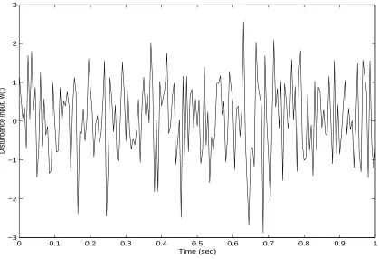
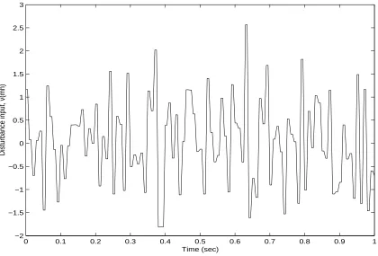
H∞ controller for system (4.1) is depicted in Fig. 1. The graphs in Fig. 2 and Fig. 3,
respectively, only show the first second of the input disturbance signals w(t)andv(mh)which were used during the simulation. The sampling time used in the simulation was 0.01 sec.
From Fig. 1, we can see that after1200seconds the ratio
n
kzk2
[0,T]+kzdk 2 (0,T)
o n
kwk2 [0,T]+kvk
2 (0,T)
o tends to a constant
value which is about 0.018. So the L2 gain from kwk[0,T]+kvk(0,T) to kzk[0,T]+kzdk(0,T) is
about
√
0.018 = 0.134, which is less than the prescribed value 1.
5
Conclusion
This paper has investigated the problem of stablising a class of fuzzy system models under sampled measurement using an H∞ fuzzy output feedback controller. A nonlinear sysyem
0 200 400 600 800 1000 1200 1400 1600 1800 2000 0
0.005 0.01 0.015 0.02 0.025
Ratio of the regulated energy to the disturbance energy
Time (sec)
Figure 1: Ratio of the regulated energy to the disturbance energy.
theory, a technique for designing an H∞ fuzzy output feedback control law which globally stabilises this class of nonlinear systems under sampled measurement has been developed. In contrast to the results given in [33, 34], the premise variables of theH∞fuzzy output feedback controller are allowed to be different from the premise variables of the Takagi-Sugeno fuzzy model of the plant.
References
[1] B. Bamieh, J. Pearson, B. Francis, and A. Tannenbaum, “A lifting technique for linear periodic systems with applications to sampled-data control,”Systems & Control Letters, vol. 17, pp. 78–88, 1991.
[2] H. T. Toivonen, “Sampled-data control of continuous-time system with anH∞
optimal-ity criterion,” Automatica, vol. 28, pp. 45–54, 1992.
0 0.1 0.2 0.3 0.4 0.5 0.6 0.7 0.8 0.9 1 −3
−2 −1 0 1 2 3
Disturbance input, w(t)
Time (sec)
Figure 2: The disturbance input, w(t).
435, 1992.
[4] Y. Yamamoto, “On the state space and frequency domain characterization ofH∞ norm of sampled-data systems,” Systems & Control Letters, vol. 21, pp. 163–172, 1991.
[5] S. Hara and P. T. Kabamba, “Worst case analysis and design of sampled-data control systems,” in Proc. of 29th IEEE Conf. Decision Contr., Honolulu, HI, pp. 202–203, 1990.
[6] P. Shi, “Robust filtering for uncertain systems with sampled measurements,” Int. J. Systems Science, vol. 27, no. 12, pp. 1403–1415, 1996.
[7] P. Shi, “Filtering on sampled-data systems with parametric uncertainty,” IEEE Trans. Automat. Control, vol. 43, 1998. to appear.
[8] W. Sun, K. M. Nagpal, and P. P. Khargonekar, “H∞ control and filtering for
sampled-data systems,” IEEE Trans. Automat. Contr., vol. 38, pp. 1162–1175, 1993.
0 0.1 0.2 0.3 0.4 0.5 0.6 0.7 0.8 0.9 1 −2
−1.5 −1 −0.5 0 0.5 1 1.5 2 2.5 3
Disturbance input, v(mh)
Time (sec)
Figure 3: The disturbance input, v(mh).
[10] N. Sivashankar and P. Khargonekar, “Characterization of theL2-induced norm for linear systems with jumps with application to sampled-data systems,” SIAM J. Control and Optimisation, vol. 32, pp. 1128–1150, 1994.
[11] P. Shi, L. Xie, and C. de Souza, “Output feedback control of sampled-data systems with parametric uncertainties,” in Proc. 31st IEEE Conf. Decision & Control, (Tucson, AZ), pp. 2876–2881, 1992.
[12] L. Xie, P. Shi, and C. E. de Souza, “On designing controllers for a class of uncertain sampled-data nonlinear systems,” IEE Proc.-Control Theory Appl., vol. 140, pp. 119– 126, 1993.
[13] P. Shi, “Controller design for uncertain systems under sampled measurements,” IMA J. Mathe. Contr. Inform, vol. 15, no. 3, pp. 1–21, 1998.
[15] Shi, P., (1998). Controller design for uncertain systems under sampled measurements.
IMA J. Mathe. Contr. Inform, 15, 133–153.
[16] Shi, P., E. K. Boukas and R. K. Agarwal, (1999). Control of Markovian jump discrete-time systems with norm bounded uncertainty and unknown delays. IEEE Trans. Au-tomat. Control, 44(11), 2139–2144.
[17] Tadmor, G., (1992). H∞optimal sampled-data control in continuous time systems. Int.
J. Control,56(1), 99–141.
[18] A. Isidori and A. Astolfi, “Disturbance attenuation and H∞- control via measurement
feedback in nonlinear systems,” IEEE Trans. Automat. Contr., vol. 37, pp. pp. 1283– 1293, 1992.
[19] S. Suzuki, A. Isidori, and T. J. Tarn, “H∞ control of nonlinear systems with sampled measurements,” J. Math. Systems, Estimation, and Control, vol. 5, pp. 1–12, 1995.
[20] H. Guillard, “On nonlinear H∞ control under sampled measurements,” IEEE Trans. Automat. Contr., vol. 42, pp. 880–885, 1997.
[21] Nguang, S. K. and P. Shi, (2000). Nonlinear H∞ filtering of sampled-data systems.
Automatica,36(2), 303–310.
[22] Nguang, S. K. and P. Shi, (2000). On design filters for uncertain sampled-data nonlinear systems. Systems & Contr. Letts, 41(2), 305–316.
[23] Cao, S. G., N. W. Ree and G. Feng, (1996). Quadratic stability analysis and design of continuous-time fuzzy control systems. Int. J. Syst. Sci.,27, 193–203.
[24] Chen, C., P. C. Chen and C. K. Chen, (1993). Analysis and design of fuzzy control system. Fuzzy Sets Systs., 57, 125–140.
[25] Nguang, S. K. and P. Shi. H∞ control of fuzzy system models using linear output
controller. Technical report. submitted for publication, 2000.
[26] Takagi, T. and M. Sugeno, (1985). Fuzzy identification of systems and its applications to modelling and control. IEEE Trans. Syst. Man. Cybern.,15, 116–132.
[28] Tanaka, K., (1995). Stability and stabiliability of fuzzy neural linear control systems.
IEEE Trans. Fuzzy Syst., 3, 438–447.
[29] Tanaka, K., T. Ikeda and H. O. Wang, (1996). Robust stabilization of a class of uncertain nonlinear systems via fuzzy control: Quadratic stabilizability, H∞ control theory, and
linear matrix inequality. IEEE Trans. Fuzzy Syst.,4, 1–13.
[30] Teixeira, M. and S. H. Zak, (1999). Stabilizing controller design for uncertain nonlinear systems using fuzzy models. IEEE Trans. Fuzzy Syst.,7, 133–142.
[31] Wang, H. O., K. Tanaka and M. F. Griffin, (1996). An approach to fuzzy control of nonlinear systems: Stability and design issues. IEEE Trans. Fuzzy Syst., 4, 14–23.
[32] Wang, L., (1997). A course in fuzzy systems and control. Englewood Cliffs, NJ: Prentice-Hall.
[33] Ma, X. J., Z. Q. Sun and Y. Y. He, (1998). Analysis and design of fuzzy controller and fuzzy observer. IEEE Trans. Fuzzy Syst., 6, 41–51.
[34] B. S. Chen, C. S. Tseng and H. J. Uang,“Mixed H2/H∞ fuzzy output feedback control