SQA by Defect prediction: An SVM based In-Appendage Software Development Log Analysis

SQA by Defect prediction: An SVM based In-Appendage

Software Development Log Analysis

N.Rajasekhar Reddy Research Scholar

Department of Computer Science and Engineering, Rayalaseema University Kurnool, Andhra Pradesh, India

M.VinayaBabu Profe ssor

Department of Computer Science and Engineering, Chalapati Institute of Engineering and Technology Guntur, AndhraPradesh, India

Abstract- The present paper proposes a Machine learning technique for defect forecasting and handling for SQA called appendage log training and analysis, can be referred as ALTA. The proposed defect forecasting of in-appendage software development logs works is to deal the forecasted defects accurately and spontaneously while developing the software. The present proposed mechanism helps in minimizing the difficulty of SQA. The overall study is conducted on evaluating the proposed model which indicates the defect forecasting in-appendage software development log training and analysis is significant growth to lessen the complexity of Software Quality Assessment.

Keywords-Hybrid software development method, conventional software development methods, agile software development methods, Software Engineering

1. INTRODUCTION

Research is being prominent in all engineering and science disciplines. To raise the quality of soft ware research has been inevitable even for software development.

According to the hierarchical models of Boehm et al. [1], for the last thirty years, a different types of models are developed to increase quality of software of which a few became standard. At present these models are being used, to specify the quality need and, to test present systems or to identify the defect density of a system in the field.

A number of varieties of models have been engendered during the last three decades and named as ―quality models‖. For instance on the spectrum of diverse models include taxonomic models like the ISO 9126 [2], metric-based models like the maintainability index (MI) [3] and stochastic models like reliability growth models (RGMs) [4]., These models seems to have less similarities though they deal with software quality. This variation is due to the purposes the models pursue: The ISO 9126 defines quality, metric-based approaches, used for assessment of the quality of a particular system and reliability growth models tells quality. In order to avoid comparison various purposes like definition, assessment and prediction of quality, to classify quality models are used. Therefore, the ISO 9126 is defined as definition model, metric-based approaches as assessment models and RGMs as prediction models. Though definition, assessment and prediction of quality are various purposes, they are certainly dependent of each other: It is very difficulty for assessing quality without knowing it‘s actually constitutes and at the same time not easy to predict quality without knowing assessment process. Quality models relation is illustrated by the DAP classification shown in Fig. 1.

Fig 1: DAP Classification [33]

The DAP classification[33] points prediction models as one of the most advanced form of quality models because they can also be utilized to define and assess quality. Hence, this opinion only applies for ideal models. Fig. 1displays that present quality models do not include all aspects equally. If we observe the ISO 9126defines quality but to assess it is possible; the MI says assessment but can not define quality. RGMs also predicts without defining quality.

2. RELATED WORK

Coming to the related works, the main forthcoming of present quality models is that they do not relate to an explicit meta model. Therefore the structure of the model elements is not clearly defined and the interpretation is left to the reader.

Quality models must be central treasure for the information about quality. So the various tasks of quality engineering should depend upon one quality model. Now days, first problem is that quality models are used separately for specification of quality needs and the assessment of software quality. Second problem is that now a day‘s quality models are not addressing various opinions on quality. For software engineering, the value-based opinion is commonly considered of high importance [5]. Which is mostly missing in existing quality models [6].

Software systems consists a large variety which ranges from a large amount of business information systems to small embedded controllers. These variations must be accounted for in quality models by defined means of customization but is lacking in the present quality models, [7, 8, and 9].

Present quality models lack clarity in defining the decomposition criteria which determine the difficult concepts of quality of decomposition. Most definition models base on a taxonomic, hierarchical decomposition of quality attributes. The decomposition model does not follow defined guidelines and can be arbitrary [10, 11, 12, 6]. Therefore, it is hard to identify similar quality attributes, like availability. In addition to large quality models, with unclear decomposition locating elements becomes difficult. Developers have to search for large parts of the model to assert that an element does not exist. This leads to redundancy because of presence of similar elements.

The vague decomposition in most of the quality models will also be the cause of overlapping in various quality attributes. In addition to, these overlaps will not be considered explicitly. I f we observe security will be influenced by availability (denial of service attack), a part of reliability; code quality factor of maintainability is considered as an indicator for security [13]. Most quality model frameworks do not give ways for utilizing the quality models for constructive quality assurance. For instance , hoe the quality models communicated to project participants is not clear. Guidelines is a common method of communicating information. Pragmatically , guidelines which are meant for communicating the knowledge of a quality model face problems, which are directly related to corresponding problems of the quality models itself; e.g. the guidelines will not be concrete enough and the document structure of the guideline will not be aligned according to anevident schema. Rationales are often not provided for the rules the guidelines impose. Other problem is that the quality models are not define tailoring methods to use the guidelines to the application area.

Unclear decomposition of quality attributes, which mentioned earlier, is one problem for analytical quality assurance. The given quality attributes are very much abstract rather than straightforward checkable in a concrete software system [3,5]. Due to the present quality models, define checkable attributes and refinement methods to get checkable attributes, they are difficult to utilize in measurement [14, 6].

In the realm of software quality, a huge number of metrics for measurement have been planned. But these metrics due to lack of structure in quality models faces problems. One such problem is that in spite of defining metrics, the quality models fail to provide a detailed account of the influence that specific metrics have on

software quality [6]. Because of poor semantics, the total of metric values along the hierarchical levels will be problematic. Other problem is that the given metrics doesn‘t possess clear motivation and validation. A part from this, present approaches do no value the fundamental rules of measurement theory and, therefore, forced to create duplicate results [15].

Because of the problems in constructive and analytical quality assurance, the possibility of certification on basis of quality models will face problems [14]. It should be stated that measurement is important for any control process. Hence the measurement quality attributes is necessary for an efficient quality assurance processes and for engineering needs.Predictive quality models don‘t possess definition of the concepts they are depend on. Many of them depend on regression using a set of software metrics. This regression results in equations that are difficult to interpret [16]. Pragmatically prediction models is context-dependent, also complicates broad application. Most factors influence the typical prediction goals and especially , factors that varies robustly. Generally in prediction models these context conditions will not be made explicitly.

Service-oriented distributed systems evolve in size and complexity, assures that they conform to their specifications throughout the software life cycle becomes hard. This origins the problem of serialized- phasing development [17], where application- level entities are devised after infrastructure-level entities. Serialized-phasing improvement builds it difficult to evaluate end-to-end functional and quality-of-service (QoS) aspects until late in the software life cycle for example, at system integration time.

Agile techniques addresses functional aspects of serialized-phasing development by authorizing software functionality throughout software life cycle[18, 19]. One such example is test-driven development and continuous integration are agile techniques that endorse functional quality by assuring that software work up to the mark. The advantage of utilizing agile techniques to develop QoS assurance of service-oriented distributed systems, despite, demonstration. Developers, hence, require new techniques to aid in exploring the indication of serialized-phasing development and enable evaluation of QoS that is considered throughout the software life cycle.

Model-driven engineering (MDE) is a favorable solution for augmenting software development of service-oriented distributed systems [20]. MDE techniques like domain-specific modeling languages (DSMLs)[21], supply developers with visual representations of abstractions that holds key domain semantics and constraints. DSMLs also supply tools that transform models into stable artifacts, like source code or configuration files that are dread and error-prone to generate manually utilizing third-generation languages. These artifacts generally are not handy in the software life cycle let a proper evaluation of end-to-end QoS properties.

3 .SQA BY DEFECT PREDICTION

mentioned as key feature of the ALTA. In defect forecasting process we adapt to machine learning technique called least square support vector machines abbreviated as LSSVM. The Defect forecasting stage of the ALTA targets the improvement of logs handy as input to train the LSSVM for better forecasting. The feature bring out process that is part of SVM training process will be carried with help of mathematical model named

Intensified worst particle based Quantum particle swarm optimization, details as follow.

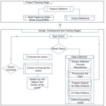
Fig 2: Defect prediction and handling using Machine Learning

Fig 3: Defect prediction Process

4. DEFECT PREDICTION USING LS-SVM[25] AND IWP-QPSO[29]

4.1 LS-SVM[25]

For solving pattern recognition and classification problem using Support vector machine (SVM) tool proposed by Vapnik[22, 23] is beneficent. . It even can be applied to regression problems by the brining up other loss function. Because of its benefits and excellent generalization performance comparing to other methods, SVM caught the attention of user and won mammoth application [5]. SVM displays extraordinary performances due to the capacity of leading global models which are special with the structural risk minimization principle [24], showing superiority over traditional empirical risk minimization principle. In addition of specific formulation, sparse solutions will be found. Linear and nonlinear regression can be performed with LSSVM. Therefore finalizing the SVM model is computationally very hard because it needs the solution of a set of nonlinear equations (quadratic programming problem). According to simplification, Suykens and

Vandewalle[25] proposed a modified version of SVM called least-squares SVM (LS-SVM[25]), that bring out in a set of linear equations in the place of a quadratic programming problem, that can be enlarge the applications of the SVM with a number of superb introductions of SVM [25, 26] and the theory of LS-SVM[25] is explained explicitly by Suykens et al[24, 25] and application of LS-SVM[25] in quantification and classification mention in a few works[27, 28].

Basically, LS-SVM[25] uses a linear relation (y = wx + b)

between the regression (x) and the dependent variable (y). The best relation is the one that reduces the cost function (Q) containing a penalized regression error term:

1 1

N

Q = wT w + γ∑ei2 ...(1) 2

2 i=1

Subject to

y

i = wTφ( x )+ b

+e i =1,..., N ...(2) ii

In the first part of cost function, weight decay useful in regularizing weight sizes and penalizes large weights. Because of regularization, the weights converge to similar value. Large weights dwindles the generalization ability of the LS-SVM [25] because of causing more variance. The regression error for all training data is in the second part of cost function the relative weight of the present part compared to the first part will be symbolized as ‗g‘ that should be used by the user.

Likewise to other multivariate statistical models, the performances of LS-SVM [25]s bases on the combination of several parameters. Attaining of the kernel function is cumbersome and it will depend on each case. Whatever, the kernel function uses more radial basis function (RBF), a simple Gaussian function, and polynomial functions where width of the Gaussian function and the polynomial degree will be used, which should be optimized by the user, to obtain the support vector. For the RBF kernel and the polynomial kernel it should be stressed that it is very necessary to do a careful model selection of the tuning parameters, in combination with the regularization constant g, in order to achieve a good generalization model.

4.2 IWP- QPSO (Intensifying the Worst Particle for QPSO)[29]

S.Nagaraja Rao et al[12] did to optimize the QPSO by intensifying worst swarm particle with new swarm particle. An interpolate equation will be traced out by applying a quadratic polynomial model on existing best fit swarm particles. Depending on emerged interpellant, new particle will be find. If the new swarm particle found as better one in comparison to least good swarm particle then substitution takes place.

The computational steps of optimized QPSO algorithm as follows:

Step 1: Initialize the swarm. Step 2: Calculate mbest Step 3: Update particles position

Step 4: Evaluate the fitness value of each particle

Step 5: If the current fitness value is better than the best fitness value (Pbest) in history Then Update Pbest by the current fitness value.

Step 7: Find a new particle

Step 8: If the new particle is better than the worst particle in the swarm, then replace the worst particle by the new particle. Step 9: Go to step 2 until maximum iterations reached. The swarm particle can be found using the fallowing.

ti =∑ pi qi ) f (r) p = a, q = b, r = c for k =1; 3

k =1 p = b, q = c , r = a for k =

p = c , q = a , r = b for k =

t1i ∑ i qi) f (r p a, q b, r c for k 1; 3

k =1 p = b, q = c , r = a for k =

p = c , q = a , r = b for k =

xi =0.5*(t t

1

i i)

In the mentioned math notations ‗a‘ is best fit swarm particle, ‗b‘ and ‗c‘ are randomly selected swarm particles xi is new swarm particle.

4.3 LS-SVM [25] Regression and QPSO based hyper parameter selection

Assume that a given training set of N data points { xt , yt }tN=1

with input data xt ∈Rd and output yt ∈ R . In feature

space LS-SVM [25] regression model take the form y (x) = wTϕ (x) + b ……… (1)

Where the input data is mapped ϕ(.)

The solution of LS-SVM[25] for function estimation is given by the following set of linear equations:

 0 1 .... 1   b  0 



K (x1, x1)+1/ C K (x1, x1)

   

1

....  α1 y1 

. . . .  . = . 

    

. . . .  . . 



K ( x1, x1)

   

1

K (x1, x1)+1/ C  α1

y 1 

…… (2)

Where K(xi ,xj ) =φ ( xi )Tφ(xj )T for i, j =1...L

And the Mercer‘s condition has been applied.

This finally results into the following LS-SVM[25] model for function estimation:

f (x ) =∑αi K (x, xi ) +b …….(3) i=1L

Where α , b are the solution of the linear system, K(.,.) represents the high dimensional feature spaces that is nonlinearly mapped from the input space x. The LS-SVM[25] approximates the function using the Eq. (3).

In present work, the radial basis function (RBF) is used as the kernel function:

k ( xi, x j)=exp(−|| x − xt ||2 /σ2)

In the training LS-SVM[25] problem, there are hyper-parameters, such as kernel width parameter σ and regularization parameter C, which may affect LS-SVM[25] generalization performance. So these parameters required perfectly in tuning of reducing the generalization error. An attempt is made to tune these parameters automatically by using QPSO.

4.4 Hyper-Parameters Selection Based on IWP-QPSO[29] To surpass the usual L2 loss results in least-square SVR, we attempt to optimize hype parameter selection.

The two key factors that finalize the optimized hyper-parameters through QPSO: First one is how to represent the hyper-parameters as the particle's position, namely encoding [13,14]. Second one is defining the fitness function, that evaluates the goodness of a particle..

4.4.1 Encoding Hyper-parameters:

The optimized hyper-parameters for LS-SVM [25] consists kernel parameter and regularization parameter. To solve hyper-parameters selection by the proposed IWP-QPSO [29], every particle represents a potential solution, called hyper-parameters combination. A hyper-parameters combination of dimension m is represented in a vector of dimension m, such

as xi = (σ, C) . The resultant Hyper-parameter optimization under

IWP-QPSO [29] can found in fallowing fig 4.

a. Fitness function:

The fitness function is the generalization performance measure. For the generation performance measure, there are some other descriptions. In the present paper, the fitness function is:

fitness = 1

…. (12) RMSE(σ,γ)

Where RMSE (σ, γ) is the root-mean-square error of predicted results, which varies with the LS-SVM [25] parameters (σ ,γ ) . When the termination criterion is met, the individual with the biggest fitness corresponds to the optimal parameters of the LS-SVM [25].

The two alternatives for stop criterion of the algorithm are: First method is that the algorithm stops when the objective function value is less than a given threshold ε; the other is that it is terminated after executing a pre-specified number of iterations. The following steps describe the IWP-QPSO [29]-

Trained LS-SVM [25] algorithm:

(1) Initialize the population by randomly generating the position vector iX of each particle and set iP = iX;

(2)Structure LS-SVM [25] by treating the position vector of each particle as a group of hyper-parameters;

(3)Train LS-SVM[25] on the training set;

(4) Evaluate the fitness value of each particle by Eq.(12), update the personal best position iP and obtain the global best position gP across the population;

(5)If the stop criterion is met, go to step (7); or else go to step (6);

(6) Update the position vector of each particle according to Eq.(7), Go to step (3);

(7)Output the gP as a group of optimized parameters.

5. RISK PREDICTION IN ALTA

This section explains the proposed algorithm for ALTA. The ALTA mainly backed by LS-SVM[25] regression that relies on IWP-QPSO[29] for feature extraction.

 _{The Development log considered into multitude tuple.}  _{Collect the resultant detailed near features of each tuple}



Submit feature matrix as input to LS-SVM[25] regression under IWP-QPSO[29], which infers the data to be used for training by generating minimal required number of support vectors.

 _{Estimate the absolute levels of the features.}

 _{Do risk prediction by evaluating the features of the current} and subsequent dependent activities of the code tuple of the current development.



Identify the risk status

6. EMPIRICAL STUDY AND RESULTS DISCUSSION The performance analysis of the proposed In-Appendage risk prediction using machine learning is done by performing wholesome study on different open source project development logs. It is opted to various logs that are of applications of various sizes ranging from low, mid to large level.

The performance of the ALTA verified by applying on development log of the Gdownloader[30], which is tiny open source application, JPCAP[31], which is tiny open source application and LUCENE[32],which is large size open source application. Empirical analysis is conducted to check the performance of ALTA is as given below.

The development, test phases and their process logs were partitioned into multitude tuple set. The extracted features from each process log tuple and generalized with IWP-QPSO, then trained with LS-SVM, then attempted to predict the risks in next tuple of actions. And then we analyzed performance of the ALTA by comparing the predicted risk ratio with actual risks of each tuple logged in process log.

The results are observed are a bit intriguing. So it is concluded that ALTA influences in risk forecasting at Development and Testing stages.

Table 1 represents the comparison of defects observed during development that are logged in process logs and predicted at In-Appendage time of development and testing. The table 1, table 2 and table 3, Fig 5, fig 6 and fig 7 represents the accuracy of ALTA in risk prediction during development and testing. From the results it is clear that ALTA is significant and reliable to forecast defects during development and testing phases of the software development.

To simplify the results analysis, each application and its log partitioned into multitude tuple set of 4 for development and 4 for testing. The results description fallows

ALTA’s performance report on tiny software development:performance of validation of ALTA on GDownloader[30] process log

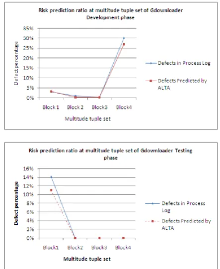
Risk prediction ratio at multitude tuple set of Gdownloader Development phase:

Block 1 Block 2 Block3 Block4

Defects in 3% 1% 0.30% 30%

Process Log

Defects 3% 0.20% 0.15% 27%

Predicted by ALTA

Risk prediction ratio at multitude tuple set of Gdownloader Testing phase:

Block1 Block2 Block3 Block4

Defects in 14% 0% 0% 0%

Process Log

Defects 11% 0% 0% 0%

Predicted by ALTA

Table 1: Comparison of defects logged in process log and defects predicted by ALTA for small size software development

Fig 5: Line chart comparison of defects logged in process log and defects predicted by ALTA for small size software development

ALTA’s performance report on medium software development:

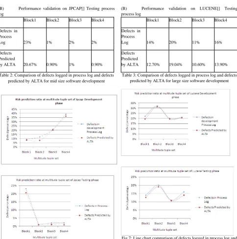
(A) Performance validation on JPCAP[31] development process log

Block Block Block3 Block4

1 2

Defects in

development

Process Log 9% 12% 21% 39%

Defects Predicted

(B) Performance validation on JPCAP[] Testing process log

Block1 Block2 Block3 Block4

Defects in Process

Log 23% 1% 2% 2%

Defects Predicted

by ALTA 20.67% 0.90% 1% 0.90%

Table 2: Comparison of defects logged in process log and defects predicted by ALTA for mid size software development

Fig 6: Line chart comparison of defects logged in process log and defects predicted by ALTA for mid size software development

ALTA’s Performance report on huge software development: (A) Performance validation on LUCENE[32] development process log

Block 1 Block 2 Block3 Block4

Defects in development

Process Log 22% 32% 20% 21%

Defects

Predicted by

ALTA 19.40% 31.10% 19.40% 20.80%

(B) Performance validation on LUCENE[] Testing process log

Block1 Block2 Block3 Block4

Defects in Process

Log 14% 20% 11% 16%

Defects Predicted

by ALTA 12.70% 19.04% 10.60% 13.90%

Table 3: Comparison of defects logged in process log and defects predicted by ALTA for large size software development

Fig 7: Line chart comparison of defects logged in process log and defects predicted by ALTA for large size software development

The results show that the performance of risk prediction in ALTA is proportional to the size of log entries. Though maximum number of log entries are entered but provides accurate results in generalizing features, Therefore the defect prediction in ALTA is accurate. With this we can come to the conclusion that ALTA as in appendage risk prediction model can lessen the cost because of defects in development and testing.

7. CONCLUSION

REFERENCES

[1] B. W. Boehm, J. R. Brown, H. Kaspar, M. Lipow, G. J. Macleod, and M. J. Merrit. Characteristics of Software Quality. North-Holland, 1978

[2] ISO. Software engineering – product quality – part 1:Quality model, 2001.

[3] D. Coleman, B. Lowther, and P. Oman. The application of software maintainability models in industrial software systems. J. Syst. Softw., 29(1):3–16, 1995.

[4] M. R. Lyu, editor. Handbook of Software Reliability Engineering. IEEE Computer Society Press and McGraw-Hill, 1996.

[5] S. Wagner. Using economics as basis for modelling and evaluating software quality. In Proc. First International Workshop on the Economics of Software and Computation (ESC-1), 2007

[6] B. Kitchenham and S. L. Pfleeger. Software quality: The elusive target. IEEE Software, 13(1):12–21, 1996.

[7] E. Georgiadou. GEQUAMO—a generic, multilayered,

cusomisable, software quality model. Software Quality Journal, 11:313–323, 2003.

[8] S. Khaddaj and G. Horgan. A proposed adaptable quality model for software quality assurance. Journal of Computer Sciences, 1(4):482– 487, 2005.

[9] J.M¨unch and M. Kl¨as. Balancing upfront definition and customization of quality models. In Workshop-Band Software- Qualit¨atsmodellierung und -bewertung (SQMB 2008). Technische Universit¨at M¨unchen, 2008.

[10] M. Broy, F. Deissenboeck, and M. Pizka. Demystifying maintainability. In Proc. 4th Workshop on Software Quality (4-WoSQ), pages 21–26. ACM Press, 2006.

[11] F. Deißenb¨ock, S. Wagner, M. Pizka, S. Teuchert, and J.-F. Girard. An activity-based quality model for maintainability. In Proc. 23rd International Conference on Software Maintenance (ICSM ‘07). IEEE Computer Society Press, 2007.

[12] B. Kitchenham, S. Linkman, A. Pasquini, and V. Nanni. The

SQUID approach to defining a quality

model. Software Quality Journal, 6:211–233, 1997.

[13] V. Basili, P. Donzelli, and S. Asgari. A unified model of dependability: Capturing dependability in context. IEEE Software, 21(6):19–25, 2004.

[14] C. Frye. CMM founder: Focus on the product to improve quality, June 2008.

[15] N. Fenton. Software measurement: A necessary scientific basis. IEEE Trans. Softw. Eng., 20(3):199–206, 1994.

[16] N. E. Fenton and M. Neil. A critique of software defect prediction models. IEEE Trans. Softw. Eng., 25(5):675– 689, 1999

[17] H.W.J. Rittel and M.M. Webber, ―Dilemmas in a General Theory of Planning,‖ Policy Sciences, vol. 4, no. 2, 1973, pp. 155–169. [18] P. Abrahamsson et al., ―New Directions on Agile Methods: A

Comparative Analysis,‖ Proc. 25th Int‘l Conf. Software Eng. (ICSE 03), IEEE CS Press, 2003, pp. 244–254.

[19] D. Saff and M.D. Ernst, ―An Experimental Evaluation of Continuous Testing during Development,‖ Proc. ACM SIGSOFT Int‘l Symp. Software Testing and Analysis, ACM Press, 2004, pp. 76–85. [20]D.C. Schmidt, ―Guest Editor‘s Introduction: Model- Driven Engineering,‖ Computer, vol. 39, no. 2, 2006, pp. 25–31. [21] G. Karsai et al., ―Model-Integrated Development of Embedded

Software,‖ Proc. IEEE, vol. 91, no. 1, 2003, pp. 145–164. [22] Cortes, C.; Vapnik, V.; Mach. Learn. 1995, 20, 273.

[23] Sun J, Xu W, Feng B, A Global Search Strategy of Quantum-Behaved Particle Swarm Optimization. In Proc. of the 2004 IEEE Conf. on Cybernetics and Intelligent Systems, Singapore: 291 – 294, 2004.

[24] Suykens, J. A. K.; Vandewalle, J.; Neural Process. Lett. 1999, 9, 293.

[25] Suykens, J. A. K.; van Gestel, T.; de Brabanter, J.; de Moor, B.; Vandewalle, J.; Least-Squares Support Vector Machines, World Scientifics: Singapore, 2002.

[26] Zou, T.; Dou, Y.; Mi, H.; Zou, J.; Ren, Y.; Anal. Biochem. 2006, 355, 1.

[27] Ke, Y.; Yiyu, C.; Chinese J. Anal. Chem. 2006, 34, 561.

[28] Niazi, A.; Ghasemi, J.; Yazdanipour, A.; Spectrochim. Acta Part A 2007, 68, 523.

[29] Dr S.Nagaraja Rao, Dr.M.N.Giri Prasad "A New Image Compression framework :DWTOptimization using LS-SVM[25] regression under IWP-QPSO[29] based hyper parameter optimization", (IJCSIS) International Journal of Computer Science and Information Security,Vol. 9, No. 7, July 2011

[30] http://sourceforge.net/projects/gdownloader/ [31] http://netresearch.ics.uci.edu/kfujii/Jpcap/doc/ [32] http://lucene.apache.org/