R E S E A R C H
Open Access
Preview tracking control for a class of
fractional-order linear systems
Fucheng Liao
1*and Hao Xie
1*Correspondence: [email protected] 1School of Mathematics and Physics, University of Science and Technology Beijing, Beijing, P.R. China
Abstract
This paper studies the preview tracking control of a class of fractional-order linear systems. Firstly, we use the fractional derivative property to take the fractional derivative of both sides of the state equation several times, and we obtain a formal ordinary linear system. An augmented error system is constructed for the transformed ordinary linear system, the appropriate performance index function is introduced and relevant results of the optimal preview control are applied to design the optimal preview controller for the augmented error system when the reference signal is previewable. Based on the relationship between the original system and the augmented error system, the preview tracking controller of the original system can be obtained. It can guarantee the asymptotic tracking of the output of the original closed-loop system to the reference signal. The validity of the theoretical results is verified by numerical simulation.
Keywords: Fractional-order linear systems; Augmented error system; Tracking control; Preview control
1 Introduction
The fractional-order system refers to the control system described by a fractional differen-tial equation. In traditional control theory, the derivatives in the control system described by ordinary differential equations are all of integer order. However, it was later discovered that many physical systems exhibit fractional kinetic behavior because of their specific material and chemical properties [1–4]. If the equations containing fractional derivatives are used to describe such a system, the essential properties of the object of study can be better revealed. Therefore, the fractional-order system theory has been propounded and applied in many fields of engineering science [5–8]. For example, in [7], by employing the spectral theorem, Duhamel’s formula is proved for the time-fractional-order Schrödinger equations, and properties of solution operators are given. Reference [8] investigates the existence, uniqueness and Hölder continuity of solutions to the time-fractional Navier– Stokes equations. In recent years, the study of fractional-order systems has been extended to the field of robust control, optimal control, sliding mode control, fault-tolerant control, iterative learning control and other advanced control strategies [9–18]. Reference [9] stud-ies the static output feedback control problem of fractional uncertain systems by using the linear matrix inequality method. In Refs. [10–12], the variational method of classical op-timal control is extended to fractional-order systems, and the Euler–Lagrange equation of
fractional-order variational problems is obtained. The variational method and Lagrange multiplier method are combined to solve the equations numerically. In [13], a sliding mode controller is designed for fractional-order linear systems, a new fractional-order switching surface is proposed, and the case with input delay and state delay is considered. In [14], the problem of robust fault-tolerant control for continuous-time fractional-order systems with interval parameters and sensor faults is studied by establishing sensor fault model and state observer. Based on the properties of fractional derivative and generalized Gronwall inequality, a P-type iterative learning control updating laws for a class of delay fractional-order systems is given in [15]. In [16], aPDα-type distributed iterative learning control laws
is proposed for consensus tracking of nonlinear fractional multi-agent systems. Reference [17] discusses the problem of complete tracking for a class of fractional-order systems in a finite-time interval, and gives fractional-order iterative learning control laws involving a local average operator associated with probability. In addition, the fractional-order sys-tem has been successfully applied to the design of the fractional-order damper, antilock braking systems, and other practical engineering problems [19–21].
In many practical cases, the future reference signal or the future disturbance signal of the control system is partly or completely known, such as the flight path of aircraft, the pro-cessing path of numerically-controlled machine tools, the driving path of vehicles, and so on. The future information can be used to design the controller to improve the con-trol quality of closed-loop systems. Such problems are problems of preview concon-trol. Since Sheridan put forward the concept of preview control in the 1960s, it has received exten-sive attention and formed a relatively complete set of theories and methods. At present, preview control has made progress in the theoretical studies of integer-order systems such as continuous-time linear systems, random systems and multi-agent systems. In [22], the problem of optimal preview control for continuous-time systems is studied by using the augmented system method. On the basis of [22], [23] studies the situation in which both reference signal and disturbance signal can be previewed at the same time. Reference [24] studies the coordinated optimal preview tracking control problem for continuous-time multi-agent systems on directed graphs. In [25], the optimal preview control problem for a class of continuous-time stochastic systems is studied by constructing an auxiliary sys-tem. At the same time, preview control is being applied successfully to many engineering control problems such as vehicle active suspension systems, electromechanical servo sys-tems, robots, and aircraft [26–28].
the-ory of fractional-order systems. The conclusions and methods of fractional-order systems can be directly applied to ordinary control systems.
The research contents are arranged as follows. Section1is the introduction. Section2 provides a few basic concepts, for completeness. Section3presents the problem of preview control for fractional-order linear systems. The problem of preview controller design for such systems is discussed in Sect.4. Sections5and6discuss the conditions under which the controller exists. Section7is for a numerical simulation. Finally, Sect.8is for a brief conclusion.
2 Preliminaries
In its theoretical development, many definitions of fractional-order calculus have emerged because of different angles of study. The scientific rationality of the definitions has been convincingly tested in practice. The definitions used in this article are described below and related properties are given. Additional definitions and properties of fractional-order calculus can be found in [29–31].
Definition 1(Fractional-order integral [29]) For anyα∈C,Re(α) > 0, the orderαintegral of the functionf(t) is defined as
t0D
–α
t f(t) = 1 Γ(α)
t
t0
(t–τ)α–1f(τ)dτ, (1)
whereΓ(α) =0∞e–ttα–1dt.
Remark1 t0D
α
t denotes the fractional integral operator,tis the independent variable,t0is
the lower boundary of the variable.
Definition 2(Caputo fractional derivative [29]) Setnas a positive integer andf(t) as a differentiable function of ordern. Whenn– 1 <α<n, the Caputo derivative of orderαin
f(t) is specified as
C t0D
α
tf(t) =t0D
–(n–α)
t
Dnf(t)
= 1
Γ(n–α) t
t0
(t–τ)n–α–1f(n)(τ)dτ. (2)
Remark2 (1)Dndenotes the derivative operator of integral order, i.e.,Dnf(t) =f(n)(t);
(2) from Definition2, it can be seen that the orderα Caputo derivative off(t) is to take the ordernderivative off(t) first, then the ordern–αintegral; (3) similarly, whenn– 1 <α<n, the function that has the derivative ofα must be the ordernderivative first; (4) lim
α→n–
C t0D
α
tf(t) =f(n)(t) [29].
Property 1([29]) The operation of the Caputo fractional derivative is linear, i.e., for ar-bitrary constantsλ1,λ2,
C t0D
α
t
λ1f1(t) +λ2f2(t)
=λ1Ct0D
α
tf1(t) +λ2Ct0D
α
Property 2([29]) Letk,m,sall be positive integers, andk+s≤m,f(t)∈C1[0,T], where
Remark3 For simplicity, we writeC
0D the compound formula of fractional integration and equal-order Caputo fractional deriva-tive calculation is
and all the above properties can be proved to be correct.
The following two lemmas need to be used in this article.
Lemma 1([32]) (A,B)is stabilizable(controllable)if and only if the matrix[λI–A B]
has full row rank for allλ∈ ¯C+(for allλ),C¯+is the closed right-half complex plane.
Lemma 2([32]) (A,B)is controllable if and only if for any eigenvalueλof A and the cor-responding left eigenvector x,we have x∗B= 0,where x∗represents the conjugate transpose of vector x.
3 Problem formulation
Consider a fractional-order linear system
C
Letyd(t)∈Rpbe the desired tracking, or reference signal. Define the difference between the reference signal and the output signal as the error signale(t), i.e.,
e(t) =y(t) –yd(t). (7)
Assumption 1 (Am,B) is stabilizable.
Assumption 2 The matrix [AmB
C 0] has full row rank.
Assumption 3 (C,Am) is detectable.
Assumption 4 The reference signalyd(t) is a piecewise-continuously differentiable
func-tion satisfying
lim
t→∞yd(t) =y¯d, tlim→∞˙yd(t) = 0, (8)
wherey¯dis constant vector. Furthermore, the reference signal is previewable, namely, the future value ofyd(τ) is available in{τ|t≤τ ≤t+lr}at each instant of timet, wherelris the preview length.
Remark5 Consider an ordinary system{xy˙((tt) =) =CxAmx(t)(t) +Bu(t): Assumption1is equivalent to
say-ing that the system is stabilizable, and Assumption3is equivalent to saying that the system is detectable. This indicates that the fractional-order control system we consider has some internal relationship with the ordinary control system. In fact, based on this relationship, we can apply the preview control theory of ordinary systems to solve the design problem of the fractional-order system controller.
This paper aims at designing a controller to allow the output of System (6a)–(6b) to asymptotically track the reference signal, or to make the error signal asymptotically ap-proach the zero vector. System (6a)–(6b) will be transformed into one that can design the controller through the optimal preview control method so as to achieve this goal.
4 System transformation and its optimal tracking controller
Firstly, we use properties 1 and 2 of the Caputo fractional derivatives to transform System
(6a)–(6b) and obtain a formal ordinary control system. Taking notice ofC0D
k
then substitute (6a) into the right side of the above equation and get
C
Denote
Equation (11) can be expressed as
˙
x(t) =Ax¯ (t) +Bv¯ (t). (12)
Obviously, the problem is transformed into one of designing the appropriate controller for System (12) so that the outputy(t) =Cx(t) of its closed-loop system can asymptotically track the reference signalyd(t). For this purpose, a quadratic performance index function is taken for System (12),
J=1 thev˙(t) is introduced in the performance indicator function, which allows the integrator to be included in the controller, thus helping to eliminate static errors [23].
Then, adopting the methods of preview control theory, an augmented error system is constructed to transform the tracking problem into a regulation problem.
Differentiating both sides of (7), we have
˙
e(t) =y˙(t) –y˙d(t) =Cx˙(t) –˙yd(t). (14)
Differentiating both sides of (12), there is
d
dtx˙(t) =A¯x˙(t) +B¯v˙(t). (15)
Combining (14) and (15) we get
˙
Equation (17) is the augmented error system we need. The basic idea to solve the prob-lem is to design the controller for System (17) through the method of optimal preview control, then obtain the controller of (12), which is the controller of System (6a)–(6b). It is not difficult to see that if we can design a state feedback to make part of componente(t) of System (17) asymptotically stable to the zero vector, our goal is achieved. It is well known from optimal control theory that the controller which minimizes the performance index function given in Equation (13) allows the closed-loop system to have this property.
Using the relevant variable in (17), we can represent the quadratic index (13) as follows:
J=1 2
∞
0
XT(t)QX˜ (t) +v˙T(t)R˙v(t)dt, (18)
whereQ˜ =C˜TQ
eC˜ = [Qe0 00]∈R(n+p)×(n+p).
It is noted that System (17) is similar in form to the system of [23], and the performance index function (18) is also similar in form to the literature [23]. Therefore, employing a similar derivation from the literature [23], the following theorem can be obtained.
Theorem 1 Suppose(A˜,B˜)is stabilizable, (Q˜1/2,A˜)is detectable,and Assumption4holds.
Let x(t) = 0,v(t) = 0and yd(t) = 0for t< 0.Then,the optimal input of the system(12)with
the minimum of the performance index function of(13)is
v(t) = –Ke t
0
e(σ)dσ–Kx
x(t) –x(0)+R–1B˜T
lr
0
expσA˜TcPDy˜ d(t+σ)dσ, (19)
where
˜
Ac=A˜ –BR˜ –1B˜TP (20)
is stable,P is the unique semidefinite solution of the following algebraic Riccati equation:
˜
ATP+PA˜ –PBR˜ –1B˜TP+Q˜ = 0. (21)
In addition,Ke=R–1B˜TPe,Kx=R–1B˜TPx,P= [Pe Px].
5 The condition that the controller exists
In this section, we discuss the condition that the controller exists, that is, the condition of Theorem1is satisfied when the original system (6a)–(6b) satisfies the desired condition, rendering (A˜,B˜) stabilizable and (Q˜1/2,A˜) detectable.
Lemma 3([23]) The pair(A˜,B˜)is stabilizable(controllable)if and only if(A¯,B¯)is stabi-lizable(controllable)and[A¯ B¯
C0]has full row rank.
The proof of Lemma3is shown in the literature [23].
Theorem 2 If(Am,B)is stabilizable(controllable),then(A¯,B¯) (that is, (Am,B¯))is
Proof We know from the obvious inequality
rank λI–Am Am–1B Am–2B · · · AB B≥rank λI–Am B
that if [λI–Am B] has full row rank, then [λI–A¯ B¯], or
λI–Am Am–1B Am–2B · · · AB B
is full row rank. The conclusion of the present theorem is obtained from Lemma1.
According to Lemma3and Theorem2, the following theorem holds.
Theorem 3 If Assumption1and Assumption2hold together,then(A˜,B˜)is stabilizable.
Proof We know from the obvious inequality
rank
¯
A B¯
C 0
=rank
Am Am–1B Am–2B · · · AB B
C 0 0 · · · 0 0
≥rank
Am B
C 0
that when Assumption 2is true, the matrix [A¯ B¯
C0] has full row rank. Besides, we know
from Theorem2that when Assumption1holds, (A¯,B¯) is stabilizable. Then, according to Lemma3, (A˜,B˜) is stabilizable when both Assumption1and Assumption2are true.
Theorem3is proved.
Theorem 4 If Assumption3is true and Qeis a positive definite matrix,then(Q˜1/2,A˜)is
detectable.
SinceA¯ =Am, this is a result of the literature [23]. To sum up, the main theorem in this paper is obtained.
Theorem 5 Suppose Assumption1–Assumption4are all true and Qeis a positive definite
matrix.Let x(t) = 0,u(t) = 0and yd(t) = 0for t< 0.Then,the input of System(6a)–(6b)
with the minimum of the performance index function of(13)is
u(t) = –Keu t
0
e(σ)dσ–Kxu
x(t) –x(0)+Ku lr
0
expσA˜TcPDy˜ d(t+σ)dσ, (22)
where
Ke=
Keu
Ke2
, Kx=
Kxu
Kx2
,
R–1B˜T=
Ku
Ku2
, Keu∈Rr×p, Kxu∈Rr×n, Ku∈Rr×(p+n).
P is the unique semi-positive definite solution of the Riccati equation(21).In addition,
Ke=R–1B˜TPe, Kx=R–1B˜TPx, P= Pe Px
Proof According to Theorem3and Theorem4, when Assumption1, Assumption2, and Assumption3are all true, (A˜,B˜) is stabilizable and (Q˜1/2,A˜) is detectable. Therefore, when
the assumptions of this theorem are satisfied, all of the conditions of Theorem1are sat-isfied. The optimal input of System (12) is obtained from Theorem1as shown in (19). Further, the first component vector of (19) is taken out and the input of System (6a)–(6b) is obtained.
To do this, dividing the matrixKe,KxandR–1B˜Tinto blocks, namely,
Ke=
Keu
Ke2
, Kx=
Kxu
Kx2
, R–1B˜T=
Ku
Ku2
,
Keu∈Rr×p, Kxu∈Rr×n, Ku∈Rr×(p+n),
we substitute them into (19), take the first row on both sides of the equal sign, and get (22),
so Theorem5can be proved.
6 A little discussion
Remark5has indicated that the tracking problem studied in this paper is closely related to ordinary systems{xy˙((tt) =) =CxAmx(t)(t) +Bu(t). This section further discusses the relationship between
the problem and system{xy˙((tt) =) =CxAx((tt)) +Bu(t). One result follows.
Theorem 6 A necessary condition for(Am,B)to be able to control is that(A,B)is
control-lable.
Proof Using contradiction, let (Am,B) be controllable. According to Lemma2, if (A,B) is uncontrollable, there must be a vectorw= 0 and a complex numberλfor
w∗A=λw∗, w∗B= 0.
Repeating right multiplicationAforw∗A=λw∗m– 1 times to get
w∗Am=λmw∗,
we have
w∗Am=λmw∗, w∗B= 0.
This is in contradiction with (Am,B) being controllable. Therefore, (A,B) is controllable. Furthermore, is the inverse of Theorem6true? The answer is no. For example, take
A= ⎡ ⎢ ⎢ ⎢ ⎣
0 1 0 0
0 0 1 0
0 0 0 1
0 0 0 0
⎤ ⎥ ⎥ ⎥
⎦, B= ⎡ ⎢ ⎢ ⎢ ⎣ 0 0 0 1 ⎤ ⎥ ⎥ ⎥ ⎦.
By utilizing Lemma 1, it is seen that (A,B) is controllable, but (A2,B) is
According to the dual principle, Theorem7is obtained from Theorem6.
Theorem 7 The necessary condition for(C,Am)to be observable is that(C,A)is
observ-able.
Theorem6and Theorem7are only necessary, but they are also meaningful. Because, if (A,B) cannot be controlled, (Am,B) must not be controlled; if (C,A) is unobservable, then (C,Am) must be unobservable. This provides some reference for us to judge the condition of Theorem1.
7 Numerical simulation
7.1 Numerical simulation algorithm
In this section, the numerical solution of Eq. (6a) is discussed. The initial statex(0) is known.
Firstly, the initial value problem of (6a) is transformed into the initial value problem of
the corresponding integral equation. By applying0D –m1
t to both sides of (6a), we can obtain
0D
Utilizing Property3, the above formula is further reduced to
x(t) =x(0) + 1 Γ(1/m)
t
0
(t–τ)m1–1Ax(τ) +Bu(τ)dτ. (24)
Equation (24) is the integral equation corresponding to fractional differential (6a). It is well known that (6a) is the same as (24) in solution, so we only need to solve the integral equation (24) [31].
Taking the sampling interval ash, the interval [0,kh] is divided intokequal points. We solve (24) on the interval [0,kh]. We obtain from Eq. (24)
=x(0) + 1
and let us take the integral
bik=mh (k– (i+ 1))m1 will lose a lot of effective numbers and thus generate large errors. Therefore, we use the results of the following transformation:
bik=
Further, by the properties of the integral, we have
kh
Substituting (31) into (29),
Letk= 1, 2, . . . , we can obtain a numerical solution. Note that the input is (22) and the final iteration format is obtained. We have
⎧
Remark6 Let us show that the results of this paper take ordinary control system (m= 1) as a special case. Whenm= 1, System (6a)–(6b) becomes
⎧
At this time, whatever the value ofiandk, alwaysbik=h, Therefore, the first formula of iteration format (33) is
x(k+ 1)h=x(0) +
This is precisely the result of the discretization of System (34) by the Euler method.
7.2 Simulation case
In this section, the effectiveness of the designed controller is verified by numerical simu-lation. Two examples are given here.
Example1 According to Ref. [1], a class of viscoelastic systems can be represented by the following fractional differential equations:
⎧
whereM,ηandkrepresent mass, damping coefficient, and elastic coefficient, respectively,
x(t) is the displacement function, andu(t) is the input quantity.
Selecting a set of state variables
and we use Eq. (35) to get
The three expressions of (36) and (37) are written as matrix vectors, namely
C
The reference signal is set as
yd(t) =
Since the reference signal is piecewise-continuously differentiable, all the conditions of Theorem5are satisfied.
the feedback gain matrix of the controller are obtained:
P= ⎡ ⎢ ⎢ ⎣
2.715493353897455 3.035936029440240 –1.242510196107315 1.608803950946188 0.236743393846281 3.035936029440240 5.685568170113166 –2.392087410321241 2.407705257751323 0.950278182238873 –1.242510196107315 –2.392087410321241 3.136796987702080 –2.938618940017380 0.826127889263837 1.608803950946188 2.407705257751323 –2.938618940017380 2.969986982371575 –0.838897582427755 0.236743393846281 0.950278182238873 0.826127889263837 –0.838897582427755 0.978748459579978
⎤ ⎥ ⎥ ⎦,
Keu= 0.717850060356720,
Kxu=
0.786609803962952 –1.918795674136359 1.941185203088351 –0.906411798984001,
Ku= 0 0 0 0.517241379310345 –0.482758620689655
.
The step lengthh= 0.01 is selected and the tracking effect is shown in Fig.1. Figure2 shows the tracking error of the system output to the reference signal under different pre-view lengths.
It can be seen from Fig.1that the output of the closed-loop system can track the ref-erence signal by taking different preview lengths. In fact, the adjustment time is 20.24 s, 18.82 s, and 17.90 s, respectively. As can be seen from Fig.2, the tracking error decreases with the increase of the preview length.
Example2 Consider the fractional-order system (6a)–(6b), where
m= 3, A=
1 1
0 –4
, B=
2 0
, C= 1 1
.
After verification, (A3,B) can be stabilized, (C,A3) can be observed, and the matrix [A3B C 0]
has full row rank. Let
Qe= 1, R= 10I3.
Figure 2The tracking error of System (38)
The reference signal is taken as a step function
yd(t) = ⎧ ⎨ ⎩
0, t< 10,
1, t≥10.
(40)
Notice thatyd(t) is piecewise-continuously differentiable, so all of the conditions of The-orem5are satisfied.
We also carried out numerical simulations for three caseslr= 0,lr= 1.5 andlr= 3.5. Respectively, the solutions of the Riccati equation and the feedback gain matrix of the controller are
P= ⎡ ⎢ ⎣
1.630667100202825 0.912870929175287 0.202762262890926 0.912870929175287 2.321921924271059 0.475792303348216 0.202762262890926 0.475792303348216 0.097691175263477 ⎤ ⎥ ⎦,
Keu= 0.182574185835057,
Kxu= 0.464384384854212 0.095158460669643
,
Ku= 0 0.2000000000000000 0
.
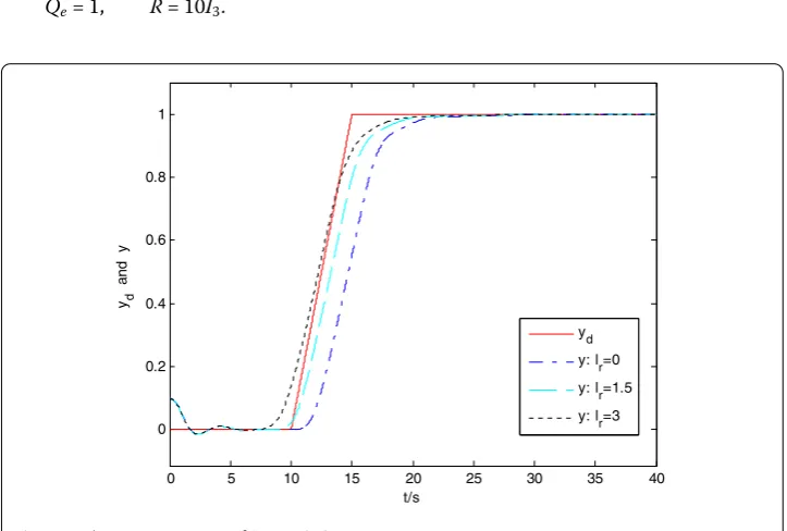
Selecting the constant step lengthh= 0.01, the initial value is set asx(0) = [0 0.05]T. The tracking effect is shown in Fig.3. It can be seen from Fig.3that the overshoot and the adjustment time decrease as the preview length increases. It is known that the adjustment time of the three cases is 22.75 s, 21.63 s and 21.36 s, respectively. Similarly, as the preview length increases, the overall tracking error gradually decreases.
Figure 3The step response of the system in Example2
Figure 4The step responses of the system in Example2for different preview lengths
output response curves oflr= 5 andlr= 20 are completely identical, and only the output response oflr= 3 is slightly different. It can be seen from Figs.3and4that all features of the preview control theory of ordinary systems are completely retained in the preview control of fractional-order systems.
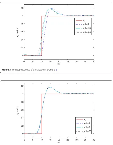
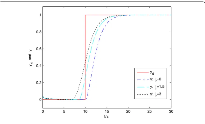
In Example2, whenm= 1 is the ordinary control system, let
Qe= 1, R= 13.
Figure 5The step response of an ordinary system
The three cases oflr= 0,lr= 1.5 andlr= 3.0 are numerically simulated. The solution of the Riccati equation and the feedback gain matrix of the controller are obtained:
P= ⎡ ⎢ ⎣
2.618310767549180 1.802775637731997 0.835457432601274 1.802775637731997 7.970226863749043 1.945657640326236 0.835457432601274 1.945657640326236 0.549679396948806 ⎤ ⎥ ⎦,
Keu= 0.277350098112615,
Kxu= 1.226188748269084 0.299331944665575
,
Ku= 0 0.153846153846154 0
.
Selecting the step lengthh= 0.01, the initial value isx(0) = [0 0.05]T. The tracking effect is shown in Fig.5.
Figure5shows that increasing the preview length can shorten the adjustment time and reduce overshoot. The calculation shows that the adjustment time is 17.18 s, 15.92 s and 15.42 s, respectively. Thus, up to now, the ordinary system preview control theory is a special case of the fractional system preview control theory. The conclusion and method of fractional-order systems can be directly applied to ordinary control systems.
8 Conclusion
also given in the paper. It is shown that the preview controller of the ordinary integer-order system is a special case of the preview controller of fractional-integer-order systems given in this paper. Numerical simulation shows that the designed controller is very effective.
Acknowledgements
The authors sincerely thank the referees and the editors for their helpful comments and suggestions.
Funding
This work was supported by National Key R&D Program of China (2017YFF0207401) and the Oriented Award Foundation for Science and Technological Innovation, Inner Mongolia Autonomous Region, China (No. 2012).
Availability of data and materials
Data sharing is not applicable to this article as no datasets were generated or analyzed during the current study.
Ethics approval and consent to participate Not applicable.
Competing interests
The authors declare to have no potential conflicts of interest with respect to the research, authorship, and publication of this article.
Consent for publication Not applicable.
Authors’ contributions
All authors equally contributed in the preparation of this manuscript. All authors read and approved the final manuscript.
Publisher’s Note
Springer Nature remains neutral with regard to jurisdictional claims in published maps and institutional affiliations.
Received: 30 April 2019 Accepted: 4 November 2019
References
1. Bagley, R.L., Torvik, P.J.: On the fractional calculus model of viscoelastic behavior. J. Rheol.30(1), 133–155 (1986) 2. Skaar, S.B., Michel, A.N., Miller, R.K.: Stability of viscoelastic control systems. IEEE Trans. Autom. Control33(4), 348–357
(1988)
3. Chen, Y., Moore, K.L.: Analytical stability bound for a class of delayed fractional-order dynamic systems. Nonlinear Dyn.29(1–4), 191–200 (2002)
4. Bassiouny, E., Abouelnaga, Z., Youssef, H.M.: One-dimensional thermoelastic problem of a laser pulse under fractional order equation of motion. Can. J. Phys.95, 464–471 (2017)
5. Carpinteri, A., Mainardi, F.: Fractals and Fractional Calculus in Continuum Mechanics. Springer, Wien (1997) 6. Atanackovic, T.M., Pilipovic, S., Stankovic, B., Zorica, D.: Fractional Calculus with Applications in Mechanics: Wave
Propagation, Impact and Variational Principles. Wiley, London (2014)
7. Zhou, Y., Peng, L., Huang, Y.: Duhamel’s formula for time-fractional Schrödinger equations. Math. Methods Appl. Sci.
41(17), 8345–8349 (2018)
8. Zhou, Y., Peng, L., Huang, Y.: Existence and Hölder continuity of solutions for time-fractional Navier–Stokes equations. Math. Methods Appl. Sci.41(17), 7830–7838 (2018)
9. Lan, Y., Zhou, Y.: LMI-based robust control of fractional-order uncertain linear systems. Comput. Math. Appl.62(3), 1460–1471 (2011)
10. Agrawal, O.P.: A general formulation and solution scheme for fractional optimal control problems. Nonlinear Dyn.
38(1), 323–337 (2004)
11. Agrawal, O.P.: Formulation of Euler–Lagrange equations for fractional variational problems. J. Math. Anal. Appl.272(1), 368–379 (2002)
12. Agrawal, O.P., Baleanu, D.: A Hamiltonian formulation and a direct numerical scheme for fractional optimal control problems. J. Vib. Control.13(9–10), 1269–1281 (2007)
13. Si-Ammour, A., Djennoune, S., Bettayeb, M.: A sliding mode control for linear fractional systems with input and state delays. Commun. Nonlinear Sci. Numer. Simul.14(5), 2310–2318 (2009)
14. Song, X., Shen, H.: Fault tolerant control for interval fractional-order systems with sensor failures. Adv. Math. Phys.
2013, 1–11 (2013)
15. Li, Y., Jiang, W.: Fractional order nonlinear systems with delay in iterative learning control. Appl. Math. Comput.257, 546–552 (2015)
16. Luo, D., Wang, J., Shen, D.:PDα-type distributed learning control for nonlinear fractional-order multiagent systems.
Math. Methods Appl. Sci.42(13), 4543–4553 (2019)
17. Liu, S., Wang, J.: Fractional order iterative learning control with randomly varying trial lengths. J. Franklin Inst.354(2), 967–992 (2017)
18. Liu, S., Debbouche, A., Wang, J.: ILC method for solving approximate controllability of fractional differential equations with noninstantaneous impulses. J. Comput. Appl. Math.339, 343–355 (2018)
20. Ikeda, F., Kawata, S., Watanabe, A.: An optimal regulator design of fractional differential systems. Trans. Soc. Instrum. Control Eng.37(9), 856–861 (2009)
21. Tang, Y., Zhang, X., Zhang, D., Zhao, G., Guan, X.: Fractional order sliding mode controller design for antilock braking systems. Neurocomputing111, 122–130 (2013)
22. Katayama, T., Hirono, T.: Design of an optimal servomechanism with preview action and its dual problem. Int. J. Control45(2), 407–420 (1987)
23. Liao, F., Tang, Y., Liu, H., Wang, Y.: Design of an optimal preview controller for continuous-time systems. Int. J. Wavelets Multiresolut. Inf. Process.9(4), 655–673 (2011)
24. Liao, F., Lu, Y., Liu, H.: Cooperative optimal preview tracking control of continuous-time multi-agent systems. Int. J. Control89(10), 2019–2028 (2016)
25. Wu, J., Liao, F., Tomizuka, M.: Optimal preview control for a linear continuous-time stochastic control system in finite-time horizon. Int. J. Syst. Sci.48(1), 129–137 (2017)
26. Li, P., Lam, J., Cheung, K.C.: Multi-objective control for active vehicle suspension with wheelbase preview. J. Sound Vib.
333(21), 5269–5282 (2014)
27. Yim, S.: Design of preview controllers for active roll stabilization. J. Mech. Sci. Technol.32(4), 1805–1813 (2018) 28. Takase, R., Hamada, Y., Shimomura, T.: Aircraft gust alleviation preview control with a discrete-time LPV model. SICE J.
Control Meas. Syst. Integr.11(3), 190–197 (2018)
29. Wu, Q., Huang, J.: Fractional Calculus. Tsinghua University Press, Beijing (2016) 30. Podlubny, I.: Fractional Differential Equations. Academic Press, San Diego (1999)
31. Diethelm, K.: The Analysis of Fractional Differential Equations: An Application-Oriented Exposition Using Differential Operators of Caputo Type. Springer, Berlin (2011)