R E S E A R C H
Open Access
Filtering and identification of a state space
model with linear and bilinear interactions
between the states
A Al-Mazrooei
1*, J Al-Mutawa
2, M El-Gebeily
2and R Agarwal
2,3*Correspondence:
1Department of Mathematics,
Taibah University, Al-Madinah, Kingdom of Saudi Arabia Full list of author information is available at the end of the article
Abstract
In this paper, we introduce a new bilinear model in the state space form. The evolution of this model is linear-bilinear in the state of the system. The classical Kalman filter and smoother are not applicable to this model, and therefore, we derive a new Kalman filter and smoother for our model. The new algorithm depends on a special linearization of the second-order term by making use of the best available information about the state of the system. We also derive the expectation
maximization (EM) algorithm for the parameter identification of the model. A Monte Carlo simulation is included to illustrate the efficiency of the proposed algorithm. An application in which we fit a bilinear model to wind speed data taken from actual measurements is included. We compare our model with a linear fit to illustrate the superiority of the bilinear model.
Keywords: bilinear state space model; Kalman filter and smoother; maximum
likelihood estimate; EM algorithm
1 Introduction
Bilinear systems are a special type of nonlinear systems capable of representing a vari-ety of important physical processes. They are used in many applications in real life such as chemistry, biology, robotics, manufacturing, engineering, and economics [–] where linear models are ineffective or inadequate. They have also been recently used to analyze and forecast weather conditions [–].
Bilinear systems have three main advantages over linear ones: Firstly, they describe a wider class of problems of practical importance. Secondly, they provide more flexible ap-proximations to nonlinear systems than linear systems do. Thirdly, one can make use of their rich geometric and algebraic structures, which promises to be a fruitful field of re-search for scientists [] as well as practitioners.
Bilinear models were first introduced in the control theory literature in s []. So far, the type of nonlinearity that is extensively treated and analyzed consists of bilinear in-teraction between the states of the system and the system input [, , ]. Aside from their practical importance, these systems are easier to handle because they are reducible to lin-ear ones through the use of a certain Kronecker product. In this work, we treat the case where the nonlinearity of the system consists of bilinear interaction between the states of the system themselves. This means that our model will be able to handle evolutions according to the Lotka-Volterra models [] or the Lorenz weather models [, , ], thus
enabling a wider and more flexible application of such models. To the best of our knowl-edge, no attempt has been made to treat such systems in the general setting presented here.
The widespread use of bilinear models motivates the need to develop their parameter identification algorithms. A lot of work exists in the literature which presents methods of estimation and parameter identification of linear and nonlinear systems [–]. The two most widely used techniques fall under the names of least square estimation and maxi-mum likelihood estimation, respectively.
The maximum likelihood estimation is computed through the well-known EM algo-rithm []. It is an iterative method that tries to improve a current estimate of the system parameters by maximizing the underlying likelihood densities. The algorithm is useful in a variety of incomplete data problems, where algorithms such as the Newton-Raphson method may turn out to be more complicated. It consists of two steps called the Expecta-tion step or the E-step and the MaximizaExpecta-tion step or the M-step; hence the name of the algorithm. This name was first coined by Dempster, Laird, and Rubin in their fundamental paper []. In this paper, we develop the EM algorithm for our bilinear system. This will necessitate also the development of a Kalman filter and smoother suitable for the nonlin-ear system at hand. The direct development of the recursions for the nonlinnonlin-ear filters is very complicated if not impossible altogether. Instead, we develop our recursions based on a linearization of the quadratic term that uses the most current state estimate available. The remainder of this article is arranged as follows. In Section , the bilinear state space model problem is stated along with underlying assumptions. In Section , we derive the bilinear Kalman filter and smoother. Section estimates the unknown parameters in the bilinear state space modelviathe EM algorithm. Section presents a simulation example that produces very satisfactory results. A real world example is given in Section .
2 The bilinear state space model
In this section, we introduce a bilinear state space model and describe a generalization of the Kalman filter and smoother to this model. Our model subsumes the well-known Lorentz- model [] for weather forecast, and the Lotka-Volterra evolution equations appear in many applications in chemistry, biology and control [, ]. Other types of bilin-ear models were investigated in [, ], where bilinbilin-earity occurs because of the interaction between the input and states of the system.
We will adopt the geometric notation as presented in [] where the matrix inner prod-uct of two random vectors is defined by
x,y=ExyT,
and
x=ExxT=x,x.
We know that
Given a sequenceY={y,y, . . . ,yt}of random vectors, the conditional expectationE(x|Y) with respect to this inner product is interpreted geometrically as the orthogonal pro-jection of the vector x in the space spanned by the vectors of Y. In particular, if x is uncorrelated with the elements of Y and if it has zero mean, then x is orthogonal to the subspace generated by Y andE(x|Y) = . We will also use the projection nota-tion
πtx:=πYx:=E(x|Y).
It is characterized by
x–πtx,z= ,
for allz∈M(Y); the closed subspace ofLof all random vectorszwhich can be written as measurable functions of the elements ofY[].
To introduce the model, let us first define the bilinear functiona:Rn×Rn→Rn(n+) by
a(x,y) = (xy,xy, . . . ,xyn,xy,xy, . . . ,xyn, . . . ,xnyn)T,
wherea(·,·) is similar to the Kronecker product function except that there is no repetition of the entries. Consider the bilinear state space model given by
xk+=Axk+Bzk+wk, ()
yk=Cxk+vk, k= , , . . . ,N, ()
wherexk∈Rnis the state vector,yk∈Rpis the measurement vector, andzk=a(xk,xk) is the bilinear term given by
zk=a(xk,xk) =x,xx, . . . ,xxn,x,xx, . . . ,xxn, . . . ,xnT.
The matrices are of appropriate dimensions,i.e.,A∈Rn×n,B∈Rn×n(n+)
andC∈Rp×p.
The uncorrelated noise corruption signalswk andvkare, as usual, assumed to be white having Gaussian distribution with zero mean and covariances Q and R, respectively, i.e.,
wk∼N(,Q), vk∼N(,R),
wk,wl=Qδkl, vk,vl=Rδkl
and
wk,vl= .
Proof Letl≤k. Then sincexl,wkare uncorrelated andE{wk}= ,wk⊥xl. This means thatE{wk|xl}= . Hence,
wk,zl=EEwka(xl,xl)|xl =EE{wk|xl}a(xl,xl) = .
The second equation can be shown in exactly the same way.
The Taylor polynomial expansion of the forma(x,x) at the pointxcan be written as follows (withz=a(x,x)):
To illustrate, supposen= , then
and
3 A bilinear Kalman filter and smoother
In this section, we will develop a Kalman filter and smoother for the bilinear system () and ().
3.1 A bilinear Kalman filter
Given a sequence of measurementsYt={y,y, . . . ,yt}, let
In order to compute equation (), we approximate the second-degree termH(xk,x) by using the most current available state estimation forxk; that is,
• In the case of prediction, we take
xk≈xk–k , soH(xk,x)≈H
• In the case of filtering, we take
By settingx=xkk, equation () becomes
zk≈zkk+zxkkxk–xkk+ H
xk–k ,xkkxk–xkk.
• In the case of smoothing, we take
xk≈xk+k , soH(xk,x)≈H
xk+k ,x
.
By settingx=xk+k , equation () becomes
zk≈zkk++zxk+k xk–xk+k + H
xk+k ,xk+k xk–xk+k .
In summary, we have the following linearization:
zk≈ztk+Vktxk–xtk, () where
Vkt=zxtk+ H
xtk±,xtk.
We also define
Ptk,k=xk–x
t
k,xk–x
t k
, ()
˙
Ptk,k=xk–x
t k,zk–z
t k
, ()
¨
Ptk,k=zk–z
t k,zk–z
t k
. ()
Theorem For the bilinear state space model defined by()and(),we have
xkk+=Axkk+Bzkk, ()
Pkk+=APkkAT+AP˙kkBT+BP˙kkTAT+BP¨kkBT+Q, ()
with
xk+k+=xkk++Kk+yk–Cxkk+,
Pk+k+= [I–Kk+C]Pkk+,
˙
Pk+k+=Pk+k+Vk+k+T,
¨
Pk+k+=Vk+k+P˙k+k+,
Kk+=Pk+k CTCPk+k CT+R–,
and
Vk+k+=zxk+k++ H
Proof Equation () is obtained by applying the conditional expectationEk(·) to ():
xkk+=Ek(xk+)
=Ek(Axk+Bzk+wk)
=AEk(xk) +BEk(zk) +Ek(wk)
=Axkk+Bzkk.
To obtain the error recursion (), we proceed as follows:
Pkk+=xk+–xkk+=(I–πk)xk+
=(I–πk)(Axk+Bzk+wk)
=Axk–xkk+Bzk–zkk+wk
=Axk–xkkAT+Bzk–zkkBT+Axk–xkk,zk–zkkBT
+Bzk–zkk,xk–xkkAT+Axk–xkk,wk+wk,xk–xkkAT
+Bzk–zkk,wk+wk,zk–zkkBT+wk =APkkAT+AP˙kkBT+BP˙kkTAT+BP¨kkBT+Q.
Now, whent=k, we derive the filtering steps. Let
ρk=yk–Ek–(yk) = (I–πk–)yk
= (I–πk–)(Cxk+vk) =yk–Cxk–k
=Cxk–xk–k +vk, k= , . . . ,N.
Then, the mean of the innovations is given by
Ek–(ρk) =πk–(I–πk–)yk= ,
and the variance
k+=ρk+
=Cxk+–xkk++vk+
=Cxk+–xkk+
CT+vk+ =CPkk+CT+R.
Also,
ρk+,yk=
yk+–ykk+,yk
=(I–πk)yk+,yk
=yk+, (I–πk)yk
which means that the innovations are orthogonal to the past measurements. On the other
From these results, we conclude thatxk+andρk+have a Gaussian joint distribution con-ditional onYk. That is,
represents the Kalman gain.
Next, we derive the recursion forPk+k+. Sincexk+–xkk+= (xk+–xk+k+) +πρk+(xk+–x
k k+) is an orthogonal decomposition,
The equation forP˙k+k+is obtained as follows:
˙
Pk+k+=xk+–xk+k+,zk+–zk+k+
=xk+–xk+k+,Vk+k+
xk+–xk+k+
=xk+–xk+k+,xk+–xk+k+Vk+k+T
=Pk+k+Vk+k+T.
Finally, forP¨k+
k+we have
¨
Pk+k+=zk+–zk+k+,zk+–zk+k+
=Vk+k+xk+–xk+k+,xk+–xk+k+Vk+k+T
=Vk+k+Pk+k+Vk+k+T
=Vk+k+P˙k+k+.
This completes the proof.
We summarize the bilinear Kalman filter as follows:
xk–k =Axk–k–+Bzk–k–,
Pk–k =APk–k–AT+AP˙k–k–BT+BP˙k–k–TAT+BP¨k–k–BT+Q, xkk=xk–k +Kk
yk–Cxk–k
, ()
Pkk= [I–KkC]Pk–k , ()
˙
Pkk=PkkVkkT,
¨
Pkk=VkkP˙kk,
Kk=Pk–k CTCPk–k CT+R–,
and
Vkk=zxkk+ H
xk–k ,xkk, k= , . . . ,N.
Also, note that the bilinear Kalman filter algorithm is a generalization of the Kalman filter for the linear case which is given in [].
3.2 A bilinear Kalman smoother
In this subsection, we will develop a Kalman smoother for the bilinear system () and (). We will use the following notation:
PNk,k=xk–x
N k,xk–x
N k
,
˙
PNk,k=xk–x
N k,zk–z
N k
,
¨
PNk,k=zk–z
N k,zk–z
N k
Lemma Let
k+={vk+, . . . ,vN,wk+, . . . ,wN}. ()
Then for≤k≤N– and with the approximation(),
L{ym}N =L{ym}k,xk+–xkk+,k+
, ()
where L{·}denotes the subspace spanned by{·}. Proof Recall that
zm=zNm+VmN
xm–xNm
,
that is,
zm–zmN∈Lxm–xNm.
Since
ym–yNm=C
xm–xNm
+vm,
L{ym}N =L{ym}N–,yN =L{ym}N–,yN–yNN– =L{ym}N–,xN–xNN–,vN
.
Similarly, since
ym+–yNm+=CAxm+–xNm++CBzm+–zNm++Cwm++vm+,
L{ym}N =L
{ym}N–,yN
=L{ym}N–,yN–yNN–
=L{ym}N–,xN––xN–N–,vN–,zN––zNN––,wN–,vN
=L{ym}N–,xN––xN–N–,vN–,vN,wN–
.
Continuing in this manner, we get ().
We state the bilinear Kalman smoother in the following theorem.
Theorem Consider the bilinear state space model()and()with xN
N and PNN as given in()and().Then for k=N– , . . . , ,we have
xNk =xkk+Jk
xNk+–xkk+, ()
where
Jk=PkkAT+P˙kkBTPkk+–.
Proof Noting the mutual orthogonality of{y}k,{xk+–xkk+}andk+and the orthogonality ofxkandk+,
xNk =πNxk=πkxk+π(xk+–xkk+)xk
=xkk+xk,xk+–xkk+xk+–xkk+–xk+–xkk+
=xkk+xk,xk+–xkk+
Pk+k –xk+–xkk+
.
Now,
xk,xk+–xkk+=xk,Axk+Bzk+wk–xkk+
=xk,Axk–xkk+Bzk–zkk
=xk–xkk,xk–xkk
AT+xk–xkk,zk–zkk
BT
=Pk
kAT+P˙kkBT. Thus,
xNk =xkk+PkkAT+P˙kkBTPkk+–xk+–xkk+ =xkk+Jk
xk+–xkk+
.
Equation () now follows by taking the projectionπN again of both sides and noting that k≤N. To derive (), we compute
PNk =xk–xNk=xk–xkk–Jkxk+–xkk+
=xk–xkk
–xk–xkk,xk+–xkk+
JkT–Jk
xk+–xkk+,xk–xkk
+JkPkk+JkT
=Pkk–( –πk)xk,xk+
JkT–Jk
xk+, ( –πk)xk
+JkPkk+J T k
=Pkk–( –πk)xk,Axk+Bzk
JkT–JkAxk+Bzk, ( –πk)xk
+JkPkk+JkT
=Pkk–PkkAT+P˙kkBTJkT–JkAPkk+BP˙kk+JkPkk+JkT =Pkk–JkPkk+JkT–JkPkk+JkT+JkPkk+JkT=Pkk–JkPk+k JkT,
which completes the proof.
The next theorem states the bilinear lag-one recursions.
Theorem Consider the bilinear state space model()and().Then
PNk+,k=APNk +BP˙kNT,
˙
Proof Using the definitions in () and (),
PNk+,k=xk+–xNk+,xk–xNk=( –πN)xk+, ( –πN)xk
=xk+, ( –πN)xk
=Axk+Bzk+wk, ( –πN)xk
=Axk, ( –πN)xk
+Bzk, ( –πN)xk
=APNk +BP˙kNT.
Also,
˙
PNk+,k=xk+–xNk+,zk–zNk
=xk+–xNk+,VkN
xk–xNk
=xk+–xNk+,xk–xNkVkNT
=PNk+,kVkNT.
4 The bilinear EM algorithm
The unknown parameter setθ={A,B,C,Q,R,V,μ}is estimated by the EM algorithm that iteratively updates the current estimateθ(i) ofθby maximizing the log-likelihood function
logL(θ,XN,YN)
=argmin
θ
logf(x–μ) + N
k=
logfw(xk–Axk––Bzk–)×fv(yk–Cxk)
, ()
where
• f(·)represents then-variate normal density of the initial statexwith meanμand the covariance matrixV.
• fv(·)represents thep-variate normal density with zero mean and the covariance matrixR.
• fw(·)represents then-variate normal density function with zero mean and the covariance matrixQ.
The conditional expectation step (E-step) finds the missing data,i.e.,XN, given the ob-served data and current estimated parameters, and then substitutes these expectations for the missing data. Specifically, letθ(i– ) be the current estimate of the parameterθ, then the E-step finds the conditional expectation E{·}of the complete-data log-likelihood givenθ(i– ):
qθ|θ(i– )= ElogL(θ,XN,YN)|YN,θ(i– ). ()
The M-step determinesθ(i) by maximizing the expected complete-data log-likelihood
qθ(i)|θ(i– )≥qθ|θ(i– ), ∀θ.
Theorem For the bilinear state space model()and(),
Proof Since the system is Markovian, we may use Bayes’ rule successively to get
p(θ,XN,YN) =p(y, . . . ,yN,x, . . . ,xN) ()
Now, substituting these densities in () and taking the logarithm of both sides, we get
L(θ,XN,YN) = –
log|V|– (x–μ)
–N
The result follows upon taking the expectation conditional onYN, making use of
EN
and simplifying. The middle equality follows from the fact that odd moments of Gaussian
random variables vanish.
Then
qθ(i)|θ(i– )=q(μ,V) +q(A,B,Q) +q(C,R) + const,
which means thatq(θ(i),θ(i– )) is maximized by separately minimizingq,q,q. This is done by setting the partial derivative ofqwith respect to each parameter equal to zero (i.e., ∂∂qx= ) and solving the resulting system of equations.
The EM algorithm for a bilinear state space model is summarized as follows.
Bilinear EM algorithm
. Initialize the EM algorithm by choosing initial values ofθ(). . Calculate the incomplete-data likelihood,logL(Yn;θ).
. Execute the E-step by using the bilinear Kalman filter and smoother in ()-() and ()-(), respectively.
. Execute the M-step using ()-() and update the estimates ofθusing (M-step) to obtainθ(i).
. Repeat Stepstountil convergence.
5 Simulation results
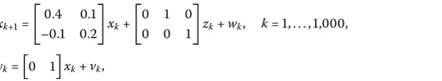
A , Monte Carlo simulation is performed to illustrate the utility of the bilinear algo-rithm. The observed data are generated according to the second-order bilinear state space model
xk+=
. . –. .
xk+
zk+wk, k= , . . . , ,, ()
yk=
xk+vk, ()
wherewkandvkare independent identically distributed (i.i.d.) Gaussian noises such that
wk∼N(, .×I), vk∼N(, .).
In all simulations, the number of iterations for the EM algorithm is fixed and its value set toJ= .
Figure shows a sample of realizations of the input noisewk, and Figure shows the output noisevk, respectively. Figure compares the observed output signals and the esti-mated output signal. The average estimates of the parameters are
A=
. . –. .
, B=
. . –. .
,
C=–. . .
The mean square error (MSE) is defined as
EN= N
N
k=
Figure 1 Input noise.
Figure 2 Output noise.
Figure 3 Observed and estimated output signals.
and its value for , run for different values ofcov(R) andcov(Q) is kept constant, which is shown in Table .
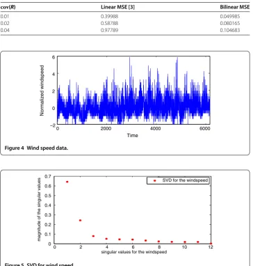
6 Application to wind speed
In this section, we apply the proposed bilinear algorithm to the daily averaged wind speed data for Arar, a city located in the north eastern region of the kingdom of Saudi Arabia for a period of years as shown in Figure . It should be noted that all the calculations are carried out on normalized time series data.
Table 1 Comparison of the mean square errors
cov(R) Linear MSE [3] Bilinear MSE
0.01 0.39988 0.049985
0.02 0.58788 0.080165
0.04 0.97789 0.104683
Figure 4 Wind speed data.
Figure 5 SVD for wind speed.
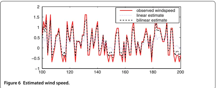
data as shown in Figure . That is, the dimension of the state equals the number of the significant singular values; heren= . For clarity, we compare the observed wind speed values with the estimated ones using a linear model [] with our proposed algorithm for a period of days as shown in Figure . The estimated parameters for the linear state space model are
A=
. . . .
, C=
. . ,
and for the bilinear state space model, they are
A=
. . . .
, C=
. . ,
B=
. –. . . .
Figure 6 Estimated wind speed.
The MSE for the estimated wind speed data using the linear EM algorithm is ., and . for the bilinear EM algorithm.
Competing interests
The authors declare that they have no competing interests.
Authors’ contributions
The authors have achieved equal contributions to each part of this paper. All authors read and approved the final version of the manuscript.
Author details
1Department of Mathematics, Taibah University, Al-Madinah, Kingdom of Saudi Arabia.2Department of Mahtematics and
Statistics, King Fahd University of Petroleum and Minerals, Dhaharan, 31261, Kingdom of Saudi Arabia.3Department of
Mathematics, Texas A&M University-Kingsville, Kingsville, TX 78363-8202, USA.
Acknowledgements
The first author was supported by Tayyebah University. The second and third authors would like to thank King Fahd University for the excellent research facilities they provide.
Received: 22 April 2012 Accepted: 24 September 2012 Published: 9 October 2012
References
1. Krener, AJ: Bilinear and nonlinear realizations of input-output maps. SIAM J. Control13(4), 827-834 (1975) 2. Pardalos, PM, Yatsenko, V: Optimization and Control of Bilinear Systems: Theory, Algorithms and Applications.
Springer, Berlin (2008)
3. Shumway, R, Stoffer, D: An approach to time series smoothing and forecasting using the EM algorithm. J. Time Ser. Anal.3(4), 253-264 (1982)
4. Strgate, SH: Nonlinear Dynamics and Chaos, with Applications to Physics, Biology, Chemistry, and Engineering. Perseus Books, New York (1994)
5. Galanis, G, Anadranistakis, M: A one-dimension Kalman filter for correction of near surface temperature forecasts. Meteorol. Appl.9, 437-441 (2002)
6. Goel, NS: On the Volterra and Other Nonlinear Models of Interacting Populations. Academic Press, San Diego (1971) 7. Lorenz, EN, Emanuel, KE: Optimal sites for supplementary weather observations: simulations with a small model. J.
Atmos. Sci.55, 399-414 (1998)
8. Lorenz, EN: Designing chaotic models. J. Atmos. Sci.62, 1574-1588 (2005)
9. Monbet, V, Ailliot, P, Prevosto, M: Survey of stochastic models for wind and sea state time series. Probab. Eng. Mech.
22, 113-126 (2007)
10. Roy, D, Musielak, ZE: Generalized Lorenz models and their routes to chaos. III. Energy-conserving horizontal and vertical mode truncations. Chaos Solitons Fractals33, 1064-1070 (2007)
11. Preistley, MB: Non-Linear and Non-Stationary Time Series Analysis. Academic Press, San Diego (1989) 12. Gibson, S, Wills, A, Ninness, B: Maximum-likelihood parameter estimation of bilinear systems. IEEE Trans. Autom.
Control50, 1581-1596 (2005)
13. Anderson, JL, Anderson, SL: A Monte Carlo implementation of the nonlinear filtering problem to produce ensemble assimilations and forecasts. Mon. Weather Rev.127, 2741-2758 (1999)
14. Bendat, J: Nonlinear System Analysis and Identification from Random Data. Wiley-Interscience, New York (1990) 15. Daum, FE: Exact finite dimensional nonlinear filters. IEEE Trans. Autom. Control31(7), 616-622 (1986)
16. Ha, QP, Trinh, H: State and input simultaneous estimation for a class of nonlinear system. Automatica40, 1779-1785 (2004)
17. Kailath, T, Sayed, A, Hassibi, B: Linear Estimation. Prentice Hall, New York (2000)
18. Kerschen, G, Worden, K, Vakakis, AF, Golinval, J: Past, present and future of nonlinear system identification in structural dynamics. Mech. Syst. Signal Process.20, 505-592 (2006)
20. Norgaard, M, Poulsen, NK, Ravn, O: New developments in state estimation for nonlinear systems. Automatica36, 1627-1638 (2000)
21. Wiener, N: Nonlinear Problems in Random Theory. MIT Press, Boston (1958)
22. Dempster, A, Laird, N, Rubin, D: Maximum likelihood from incomplete data via the EM algorithm. J. R. Stat. Soc. B39, 1-38 (1977)
23. Tanaka, H, Katayama, T: A stochastic realization algorithm via block LQ decomposition in Hilbert space. Automatica
42, 741-746 (2006)
doi:10.1186/1687-1847-2012-176