doi:10.1155/2010/969536
Research Article
Analysis and Numerical Solutions of
Positive and Dead Core Solutions of
Singular Sturm-Liouville Problems
Gernot Pulverer,
1Svatoslav Stan ˇek,
2and Ewa B. Weinm ¨uller
11Institute for Analysis and Scientific Computing, Vienna University of Technology,
Wiedner Hauptstrasse 6-10, 1040 Vienna, Austria
2Department of Mathematical Analysis, Faculty of Science, Palack´y University, Tomkova 40,
779 00 Olomouc, Czech Republic
Correspondence should be addressed to Svatoslav Stanˇek,[email protected]
Received 20 December 2009; Accepted 28 April 2010
Academic Editor: Josef Diblik
Copyrightq2010 Gernot Pulverer et al. This is an open access article distributed under the Creative Commons Attribution License, which permits unrestricted use, distribution, and reproduction in any medium, provided the original work is properly cited.
In this paper, we investigate the singular Sturm-Liouville problemuλgu,u0 0,βu1
αu1 A, whereλis a nonnegative parameter,β≥0,α >0, andA >0. We discuss the existence of multiple positive solutions and show that for certain values ofλ, there also exist solutions that vanish on a subinterval0, ρ⊂ 0,1, the so-called dead core solutions. The theoretical findings are illustrated by computational experiments forgu 1/√uand for some model problems from the class of singular differential equationsφuft, u λgt, u, udiscussed in Agarwal et al.
2007. For the numerical simulation, the collocation method implemented in our MATLAB code
bvpsuitehas been applied.
1. Introduction
In the theory of diffusion and reactionsee, e.g.,1, the reaction-diffusion phenomena are
described by the equation
Δvφ2hx, v, 1.1
wherex∈Ω⊂RN. Herev≥0 is the concentration of one of the reactants andφis the Thiele
equation satisfying the boundary conditions
βδv
δn αvA 1.2
are solutions to a boundary value problem of the type
ut ft, utφ2ht, ut,
u0 0, βu1 αu1 A, β≥0, α, A >0,
1.3
where t denotes the radial coordinate. Baxley and Gersdorff 2 discussed problem 1.3,
where f and hwere continuous and hwas allowed to be unbounded for u → 0. They
proved the existence of positive solutions and dead core solutionsvanishing on a subinterval
0, t0, 0< t0<1of problem1.3, and also covered the case of the functionhapproximated
by some regular functionhκ.
Problem1.3was a motivation for discussing positive, pseudo dead core, and dead
core solutions to the singular boundary value problem with aφ-Laplacian,
φutft, utλgt, ut, ut, λ >0, 1.4a
u0 0, βuT αuT A, β≥0, α, A >0, 1.4b
see3. Hereλis a parameter, the functionfis non-negative and satisfies the Carath´eodory
conditions on0, T×0,∞,ft,0 0 for a.e.t ∈0, T, andgis positive and satisfies the
Carath´eodory conditions on0, T× D,D 0, A/α×0,∞. Moreover, the functionft, x
is singular att0 andgt, x, yis singular atx0.
Let us denote byACloc0, Tthe set of functionsx :0, T → Rwhich are absolutely
continuous onε, Tfor arbitrary smallε >0.
A functionu ∈C10, Tis calleda positive solution of problem1.4a-1.4bifu > 0 on
0, T,φu ∈ ACloc0, T,usatisfies1.4band 1.4aholds for a.e.t ∈ 0, T. We say that
u ∈ C10, Tsatisfying1.4b isa dead core solution of problem 1.4a-1.4bif there exists a
pointρ∈ 0, Tsuch thatu 0 on0, ρ,u > 0 onρ, T,φu ∈ACρ, Tand1.4aholds
for a.e.t ∈ ρ, T. The interval0, ρis called thedead core of u. Ifu0 0,u > 0 on0, T,
φu∈ACloc0, T,usatisfies1.4band1.4aholds a.e. on0, T, thenuis calleda pseudo
dead core solution of problem1.4a-1.4b.
Since problem 1.4a-1.4b is singular, the existence results in 3are proved by a
combination of the method of lower and upper functions with regularization and sequential
techniques. Therefore, the notion of a sequential solution of problem 1.4a-1.4b was
introduced. In3, conditions on the functionsφ, f, andg were specified which guarantee
that for eachλ > 0, problem1.4a-1.4bhas a sequential solution and that any sequential
solution is either a positive solution, a pseudo dead core solution, or a dead core solution.
Also, it was shown that all sequential solutions of 1.4a-1.4b are positive solutions for
sufficiently small positive values ofλ and dead core solutions for sufficiently large values
The differential equation1.5aof the following boundary value problem satisfies all
conditions specified in3:
utγut tρ λ
1
ut
utν
, 1.5a
u0 0, αu1 βu1 1, α >0, β >0. 1.5b
Here,γ, ρ ∈ 0,∞, andν ∈ 0, γ1. We note that in papers 2,3no information on the
number of positive and dead core solutions of the underlying problem is given. In this paper, we discuss the singular boundary value problem
ut λgut, λ≥0, 1.6a
u0 0, αu1 βu1 1, α >0, β >0, 1.6b
whereλis a non-negative parameter, and the functiong ∈ C0,∞becomes unbounded at
u0. Problem1.6a-1.6bis the special case of problem1.4a-1.4b.
A function u ∈ C20,1 isa positive solution of problem1.6a-1.6b ifu satisfies the
boundary conditions1.6b,u > 0 on0,1 and 1.6aholds for t ∈ 0,1. A functionu :
0,1 → 0,∞ is calleda dead core solution of problem 1.6a-1.6b if there exists a point
ρ∈0,1such thatut 0 fort∈0, ρ,u∈C10,1∩C2ρ,1,usatisfies1.6band1.6a
holds fort ∈ ρ,1. The interval0, ρis calledthe dead core of u. Ifρ 0, thenuis calleda
pseudo dead core solutionof problem1.6a-1.6b. The aim of this paper is twofold.
1First of all, we analyze relations between the values of the parameter λ and the
number and types of solutions to problem1.6a-1.6b, provided that
g∈C0,∞, g is positive, lim
u→0gu ∞, a
0
gsds <∞ ∀a >0
1.7
or
g∈C10,∞, g is positive and decreasing, lim
u→0gu ∞, a
0
gsds <∞ ∀a >0.
2Moreover, we compute solutionsuto the singular boundary value problem
ut λ
ut, λ≥0, 1.9a
u0 0, αu1 βu1 1, α >0, β >0, 1.9b
and the singular problem1.5a,1.9b. Note that1.9ais the special case of1.6a
withgsatisfying1.8.
In 4 similar questions in context of 1.6a and the Dirichlet boundary conditions
u0 1,u1 1 have been discussed. For further results on existence of positive and dead
core solutions to differential equations of the typesu λgt, uandφugt, u, u, we
refer the reader to5–9. The Dirichlet conditions have been discussed in5–7,9, while8
deals with the Robin conditions−u−1 αu−1 a,u1 αu1 a,α,a >0.
We now recapitulate the main analytical results formulated in Theorems2.10,2.12, and
2.13. First, we introduce the auxiliary function
Hx, y:
⎧ ⎪ ⎪ ⎨ ⎪ ⎪ ⎩
αyβ y
x
ds
s
xgvdv
y
x
gvdv, 0≤x < y,
αy, 0≤xy,
1.10
whereg satisfies1.7. ByLemma 2.2, the equationHx, γx 1 has a unique continuous
solutionγ∈C0,1/α, and the function
χx:
⎧ ⎪ ⎪ ⎪ ⎨ ⎪ ⎪ ⎪ ⎩
γx
x
ds
s
xgvdv
, x∈
0,1
α
,
0, x 1
α
1.11
is continuous on0,1/α. LetM:{χx2/2 : 0< x≤1/α}. Then the following statements
hold.
iProblem1.6a-1.6bhas a positive solution if and only ifλ ∈ M. In addition, for
eacha∈ 0,1/α, problem1.6a-1.6bwithλ χa2/2 has a unique positive
solution such thatu0 a,u1 γa.
iiProblem1.6a-1.6bhas a pseudo dead core solution if and only if
λ 1
2
⎛ ⎜ ⎝
γ0
0
ds
s
0gvdv
⎞ ⎟ ⎠
2
. 1.12
iiiProblem1.6a-1.6bhas a dead core solution if and only if
λ >1
2
⎛ ⎜ ⎝
γ0
0
ds
s
0gvdv
⎞ ⎟ ⎠
2
. 1.13
In addition, for all suchλ, problem1.6a-1.6bhas a unique dead core solution.
The final result concerning the multiplicity of positive solutions to problem 1.6a
1.6b is given inTheorem 2.11. Let 1.8 hold and let Γ : max{τ : τ ∈ M}. Then Γ >
χ02/2 and for eachλ ∈χ02/2,Γ, there exist multiple positive solutions of problem
1.6a-1.6b.
In Section 2 analytical results are presented. Here, we formulate the existence and
uniqueness results for the solutions of the boundary value problem1.6a-1.6band study
the dependance of the solution on the parameter values λ. The numerical treatment of
problems 1.9a-1.9b and 1.5a-1.5b based on the collocation method is discussed in
Section 3, where for different values of λ, we study positive, pseudo dead core, and dead
core solutions of problem1.9a-1.9band positive solutions of problem1.5a-1.5b.
2. Analytical Results
2.1. Auxiliary Functions
Let assumption1.7hold, and let us introduce auxiliary functionsϕa, H, andhas
ϕax:
⎧ ⎪ ⎪ ⎨ ⎪ ⎪ ⎩
x
a
ds
s
agvdv
, x∈a,∞,
0, xa,
2.1
wherea∈0,∞,
Hx, y:
⎧ ⎪ ⎪ ⎨ ⎪ ⎪ ⎩
αyβ y
x
ds
s
xgvdv
y
x
gvdv, 0≤x < y,
αy, 0≤xy,
2.2
ht, y:αy β
1−t
y
0
ds
s
0gvdv
y
0
gvdv, t, y∈0,1×0,∞. 2.3
Here, the positive constants αandβ are identical with those used in boundary conditions
1.6b. Note that the function H is used in the analysis of positive and pseudo dead core
solutions of problem1.6a-1.6b, while the functionhfor its dead core solutions.
Properties ofϕaare described in the following lemma.
Proof. Letcbe arbitrary,c > a. Thenϕa∈Ca, c∩C1a, c, andϕais increasing ona, cby
4, Lemma 2.3where 1 is replaced byc. Sincec > ais arbitrary, the result immediately
follows.
In the following lemma, we introduce functionsγandχand discuss their properties.
Lemma 2.2. Let assumption1.7hold. Then the following statements follow.
iThe functionHis continuous onΔ {x, y∈R2: 0≤x≤y}, and∂H/∂yx, y>0 for0≤x < y.
iiFor eachx∈0,1/α, there exists a uniqueγx∈a,1/αsuch that
Hx, γx1 forx∈
0,1
α
, 2.4
andγ ∈C0,1/α,γx> xforx∈0,1/α,γ1/α 1/α.
iiiThe function
χx:
⎧ ⎪ ⎪ ⎪ ⎨ ⎪ ⎪ ⎪ ⎩
γx
x
ds s
xgvdv
, x∈
0,1
α
,
0, x 1
α
2.5
is continuous on0,1/α.
Proof. iLet us defineS, PonΔby
Sx, y:
y
x
gvdv,
Px, y:
⎧ ⎪ ⎪ ⎨ ⎪ ⎪ ⎩
y
x
ds
s
xgvdv
, 0≤x < y,
0, 0≤xy.
2.6
ThenS ∈CΔ. Letx≥0 and definem: min{gs: 0 < s ≤x1}. Then, by1.7,m >0.
Hence
0<
y
x
ds
s
xgvdv
≤ √1
m y
x
ds
√
s−x2
y−x
and consequently limx,y∈Δ,y→xPx, y 0, which means thatP is continuous atx, x. Let 0≤x0< y0. We now show thatPis continuous at the pointx0, y0. Let us choose an arbitrary
y∗in the intervalx0, y0. ThenPx, y I1x I2x, yforx∈0, y∗andy > y∗, where
I1x
y∗
x
ds
s
xgvdv
, I2
x, y
y
y∗
ds
s
xgvdv
. 2.8
Since I1 ∈ C0, y∗by 4, Lemma 2.1 where 1 was replaced by y∗, it follows that I1 is
continuous at x x0. The continuity of P at x0, y0now follows from the fact that I2 is
continuous at this point. HencePis continuous onΔ, and fromHx, y αyβPx, ySx, y
we concludeH∈CΔ. Since
∂H ∂y
x, yαβ βq
y
2xygvdv
y
x
ds
s
xgvdv
, 0≤x < y, 2.9
we have∂H/∂yx, y>0 for 0≤x < y.
iiConsider the equationHx, y 1, that is,
αyβ y
x
ds
s
xgvdv
y
x
gvdv1. 2.10
The function Hx,· is increasing on x,∞, H1/α,1/α 1, and, for x ∈ 0,1/α,
Hx,1/α>1. Hence, for eachx∈0,1/α, there exists a uniqueγxsuch thatHx, γx
1 andγ1/α 1/α. Clearly,γx> xforx∈ 0,1/α. In order to prove thatγ ∈C0,1/α,
suppose the contrary, that is, suppose thatγis discontinuous at a pointxx0,x0 ∈0,1/α.
Then there exist sequences{νn},{μn}in0,1/αsuch that limn→ ∞νn x0 limn→ ∞μn, and
the sequences{γνn},{γμn}are convergent, limn→ ∞γνn c1, limn→ ∞γμn c2,c1/c2.
Letn → ∞inHνn, γνn 1 and inHμn, γμn 1. This meansHx0, cj 1,j 1,2,
andc1c2γx0by the definition of the functionγ, which contradictsc1/c2.
iiiByii,
αγx βχx γx
x
gvdv1, x∈
0,1
α
, 2.11
γ ∈C0,1/αandγx> xforx∈0,1/α. Hence, the functionxγxgvdvis continuous
on0,1/αand positive on0,1/α. From
χx 1−αγx βxγxgvdv
, x∈
0,1
α
we now deduce thatχ∈C0,1/α. Since
χx≤ √1 m
γx
x
ds
√
s−x 2
γx−x m , x∈
0,1
α
, 2.13
wherem:min{gu: 0 < u≤1/α}>0, andχ >0 on0,1/α,γ1/α 1/α, we conclude
limx→1/α−χx 0. Henceχis continuous atx1/α, and consequentlyγ∈C1,1/α.
Letγbe the function fromLemma 2.2iidefined on the interval0,1/α. From now
on,Λdenotes the value ofγatx0, that is,
Λ γ0. 2.14
In the following lemma, we prove a property of χ which is crucial for discussing
multiple positive solutions of problem1.6a-1.6b.
Lemma 2.3. Let assumption1.8hold and let the functionχ be given by2.5. Then there exists
ε >0such that
χx> χ0, forx∈0, ε. 2.15
Proof. Note thatχ0 0Λ1/0sgvdvds. We deduce from4, Lemma 2.2with 1 replaced
byΛthat there exists anε >0 such that
Λ
x
ds
s
xgvdv
> χ0 forx∈0, ε. 2.16
Ifγx>Λfor somex∈0, ε, then2.16yields
χx
γx
x
ds
s
xgvdv
> Λ
x
ds
s
xgvdv
> χ0. 2.17
Consequently, inequality2.15holds for such anx. If the statement of the lemma were false,
then somex∗∈0, εwould exist such thatγx∗≤Λand
From the following equalities, compare2.4,
1αΛ βχ0
Λ
0
gvdv,
1αγx∗ βχx∗
γx∗
x∗
gvdv,
2.19
and fromγx∗≤Λ, we conclude that
χx∗≥χ0
Λ
0 gvdv
γx∗
x∗ gvdv
. 2.20
Finally, from
Λ
0
gvdv > γx∗
x∗
gvdv, 2.21
we haveχx∗> χ0, which contradicts2.18.
In order to discuss dead core solutions of problem1.6a-1.6band their dead cores,
we need to introduce two additional functionsμandprelated tohand study their properties.
Lemma 2.4. Assume that1.7holds and lethbe given by2.3. Then for eacht∈0,1, there exists a uniqueμt∈0,1/αsuch that
ht, μt1 fort∈0,1. 2.22
The functionμis continuous and decreasing on0,1, and the function
pt: 1
1−t
μt
0
ds s
0gvdv
, t∈0,1, 2.23
is continuous and increasing on0,1. Moreover,limt→1−pt ∞.
Proof. It follows from1.7thath∈C0,1×0,∞. Also,his increasing w.r.t. both variables,
limt→1−ht, y ∞for anyy∈ 0,1/α, and limy→0ht, y 0, limy→1/αht, y> 1 for any
t∈0,1. Hence, for eacht∈0,1, there exists a uniqueμt∈0,1/αsuch thatht, μt 1.
In order to prove thatμis decreasing on0,1, assume on the contrary thatμt1≤ μt2for
some 0 ≤ t1 < t2 < 1. Thenht1, μt1 < ht2, μt2which contradicts htj, μtj 1 for
j 1,2. Hence,μis decreasing on 0,1. Ifμwas discontinuous at a pointt0 ∈ 0,1, then
there would exist sequences{νn}and{τn}in0,1such that limn→ ∞νn t0limn→ ∞τnand
the limitsn → ∞inhνn, μνn 1 andhτn, μτn 1, we obtainht0, cj 1,j 1,2.
Consequently,c1 c2μx0by the definition of the functionμ, which is not possible.
By2.22,
αμt β
1−t
μt
0
ds
s
0gvdv
μt
0
gvdv1 for t∈0,1, 2.24
and therefore,
pt 1−αμt β0μtgvdv
, t∈0,1. 2.25
It follows from the properties ofμthat the functions 1−αμt, 1/0μtgvdvare continuous,
positive, and increasing on0,1. Hence2.25implies thatp ∈ C0,1andpis increasing.
Moreover, limt→1−pt ∞since
μt
0 1/
s
0gvdvdsis bounded on0,1.
Corollary 2.5. Let assumption1.7hold. Then
1
1−t
μt
0
ds s
0gvdv
> Λ
0
ds s
0gvdv
fort∈0,1, 2.26
and for eachλsatisfying the inequality
λ > 1
2
⎛ ⎜ ⎝
Λ
0
ds s
0gvdv
⎞ ⎟ ⎠
2
, 2.27
there exists a uniqueρ∈0,1such that
μρ
0
ds s
0gvdv
1−ρ2λ. 2.28
Proof. The equalitiesh0, y H0, yfory ∈ 0,∞andH0,Λ 1 imply thatμ0 Λ.
Since the functionpdefined by2.23is continuous and increasing on0,1, it follows that
pt> p0fort∈0,1; see2.26. Let us choose an arbitraryλsatisfying2.27. Then√2λ >
p0. Now, the properties of p guarantee that equation√2λ pt has a unique solution
ρ∈0,1. This means that2.28holds for a uniqueρ∈0,1.
2.2. Dependence of Solutions on the Parameter
λ
The following two lemmas characterize the dependence of positive and dead core solutions
Lemma 2.6. Let assumption1.7hold and letube a positive solution of problem1.6a-1.6bfor someλ >0. Also, leta:min{ut: 0≤t≤1}, andQ :max{ut: 0≤t≤1}. Thenau0,
Qu1,
Q
a
ds s
agvdv
2λ, 2.29
ut
a
ds s
agvdv
2λt fort∈0,1, 2.30
Ha, Q 1, 2.31
where the functionHis given by2.2.
Proof. Sinceu0 0 and ut λgut > 0 fort ∈ 0,1, we conclude thatu > 0 on
0,1 and a u0,Q u1. By integrating the equalityutut λgutut over
0, t⊂0,1, we obtain
ut22λ ut
a
gvdv, 2.32
and consequently, sinceu>0 on0,1,
ut 2λ ut
a
gvdv, t∈0,1. 2.33
Finally, integrating
ut ut
a gvdv
2λ, t∈0,1, 2.34
over0, tyields2.30. Now we sett1 in2.30and obtain2.29. Equality2.31follows
fromαu1 βu1 1 and from
u1 Q, u1 2λ
Q
a
gvdv Q
a
ds
s
agvdv
Q
a
gvdv. 2.35
Remark 2.7. Let1.7hold and letube a pseudo dead core solution of problem1.6a-1.6b.
Then, by the definition of pseudo dead core solutions,u0 0. We can proceed analogously
to the proof ofLemma 2.6in order to show that
Q
0
ds
s
agvdv
whereQu1, and
ut
0
ds
s
agvdv
2λt fort∈0,1, 2.37
H0, Q 1. 2.38
From2.38, we finally haveQ Λ. Consequently,u1 Λ.
Remark 2.8. Ifλ0, thenut 1/α,t∈0,1,is the unique solution of problem1.6a-1.6b. This solution is positive.
Lemma 2.9. Let assumption1.7hold and letube a dead core solution of problem1.6a-1.6bfor someλ λ0. Moreover, letQ : max{ut : 0 ≤ t ≤ 1}. ThenQ u1and there exists a point
ρ∈0,1such thatut 0fort∈0, ρ,
ut
0
ds s
0gvdv
2λ0
t−ρ fort∈ρ,1, 2.39
Q
0
ds s
0gvdv
2λ0
1−ρ, 2.40
hρ, Q1, 2.41
where the functionhis given by2.3. Furthermore,uis the unique dead core solution of problem
1.6a-1.6bwithλλ0.
Proof. Sinceuis a dead core solution of problem1.6a-1.6b withλ λ0, there exists by
definition, a pointρ∈0,1such thatu∈C10,1∩C2ρ,1,ut 0 fort∈0, ρandu >0
onρ,1. Consequently,u> 0 onρ,1, andQ u1. We can now proceed analogously to
the proof ofLemma 2.6to show that
ut 2λ0
ut
0
gvdv, t∈ρ,1, 2.42
and2.39holds. Settingt1 in2.39, we obtain2.40. Also, from1.6b,u1 Q,
u1 2λ0
Q
0
gvdv 1
1−ρ
Q
0
ds
s
0gvdv
Q
0
gvdv, 2.43
equality2.41follows.
It remains to verify thatuis the unique dead core solution of problem 1.6a-1.6b
withλ λ0. Let us suppose thatwis another dead core solution of the above problem. Let
fort∈ ρ1,1, and consequentlyw >0 onρ1,1andQ1 : max{wt : 0 ≤t ≤ 1} w1.
Hence, compare2.40and2.41,
Q1
0
ds
s
0gvdv
2λ0
1−ρ1
, 2.44
αQ1β
2λ0
Q1
0
gvdv1. 2.45
Since
αQβ2λ0
Q
0
gvdv1 2.46
by2.41, and the functionpr : αrβ2λ0
r
0gvdvis increasing and continuous on
0,∞, we deduce from2.45and 2.46thatQ Q1. Then2.40and2.44yieldρ ρ1.
Therefore, 0wt1/0sgvdvds 2λ0t−ρ fort ∈ ρ,1. Finally, sincewt 0 for
t∈0, ρand since byLemma 2.1the functionϕ0is increasing on0,∞,uwfollows. This
completes the proof.
2.3. Main Results
Let the functionχbe given by2.5and let us denote byMthe range of the functionχ2/2
restricted to the interval0,1/α,
M:
χx2
2 : 0< x≤ 1
α
. 2.47
Sinceχ∈C0,1/αbyLemma 2.2iii,χx>0 forx∈0,1/αandχ1/α 0, we can have
eitheriχx< χ0forx∈0,1/α, oriiχx1≥χ0for somex1 ∈0,1/α. Fori, we
haveM 0,χ02/2, while in case ofii,M 0,Γwith
Γ:max{τ:τ ∈ M} 2.48
holds. Clearly,Γ≥χ02/2.
Positive solutions of problem1.6a-1.6bare analyzed in the following theorem.
Theorem 2.10. Let assumption1.7hold. Then problem1.6a-1.6bhas a positive solution if and only ifλ∈ M. Additionally, for eacha∈0,1/α, problem1.6a-1.6bwithλ χa2/2has a unique positive solutionusuch thatu0 aandu1 γa.
Proof. Letube a positive solution of problem1.6a-1.6bforλ > 0. ByLemma 2.6,2.31
holds witha u0 > 0 and Q u1. Furthermore, by Lemmas2.2iiand2.6,Q γa,
1.6a-1.6bhas the unique positive solution u 1/α; see Remark 2.8. Sinceχ1/α 0,
0∈ M. Consequently, if problem1.6a-1.6bhas a positive solution, thenλ∈ M.
We now show that for eachλ ∈ M, problem1.6a-1.6bhas a positive solution, and
if λ χa2/2 for some a ∈ 0,1/α, then problem1.6a-1.6b has a unique positive
solutionusuch that u0 aand u1 γa. Let us chooseλ ∈ M. Then√2λ χafor
somea∈0,1/α. Ifa 1/α, thenχa 0. Consequently,λ0 andu1/αis the unique
solution of problem1.6a-1.6b. Clearly,u0 aandu1 γasinceaγa 1/α. Let
us suppose thata∈0,1/α. Ifuis a positive solution of problem1.6a-1.6bandu0 a,
then, byLemma 2.6; see 2.30, the equality ϕaut
√
2λt holds fort ∈ 0,1, whereϕa
is given by2.1. Hence, in order to prove that forλ χa2/2 problem1.6a-1.6bhas
a unique positive solutionusuch that u0 aandu1 γa, we have to show that the
equation
ϕaut
2λt, t∈0,1, 2.49
has a unique solution u; this solution is a positive solution of problem 1.6a-1.6b, and
u0 a,u1 γa. Sinceϕa ∈ Ca,∞∩C1a,∞,ϕais increasing by Lemma 2.1, and
ϕaγa χa,2.49 has a unique solution u ∈ C0,1. It follows from ϕaa 0 and
ϕau1
√
2λχathatua aandu1 γa. In addition,
ut
√
2λ
ϕaut
2λ
ut
a
gvdv, t∈0,1. 2.50
Hence,u∈C10,1and lim
t→0ut 0. In order to show thatuis continuous att0, we
setMmax{gs:a≤s≤1/α}>0. Then, compare2.49,
2λt
ut
a
ds
s
agvdv
≥ √1
M ut
a
ds
√
s−a 2
ut−a
M , 2.51
and therefore,
0< ut−u0
t
ut−a
t ≤
Mλt
2 , t∈0,1. 2.52
Consequently, u0 limt→0ut− a/t 0, and so u is continuous at t 0, or
equivalently,u∈C10,1. Now2.50indicates thatu∈C20,1and
ut 2λ gutu
t
2autgvdv
Moreover, by the de L’Hospital rule,
lim t→0
ut−u0
t tlim→0 ut
t tlim→0 1
t
2λ
ut
a
gvdv
2λlim t→0
gutut
2autgvdv
λlim t→0gut
λgu0.
2.54
As a resultu ∈C20,1andut λgutfort∈ 0,1. Sinceu1 γaand, by2.50,
u1 χaaγagvdv, we have
αu1 βu1 αγa β γa
a
ds
s
agvdv
γa
a
gvdvHa, γa1 2.55
byLemma 2.2ii. Thus, u satisfies1.6b, and thereforeuis a unique positive solution of
problem1.6a-1.6bsuch thatu0 aandu1 γa.
The following theorem deals with multiple positive solutions of problem1.6a-1.6b.
Theorem 2.11. Let assumption1.8hold. ThenΓ>χ02/2, withΓgiven by2.48, and for each
λ∈χ02/2,Γ, there exist multiple positive solutions of problem1.6a-1.6b.
Proof. By Lemmas 2.2iiiand 2.3,χ ∈ C0,1/α,χ1/α 0, andχx > χ0 in a right
neighbourhood ofx 0. Hence,Γ> χ02/2. Let us chooseλ∈χ02/2,Γ. Then there
exist 0 < x1 < x2 <1/αsuch thatλ χxj2/2 forj 1,2. NowTheorem 2.10guarantees
that problem1.6a-1.6bhas positive solutionsu1andu2such thatuj0 xj,j1,2. Since
x1/x2, we haveu1/u2 and therefore, for eachλ ∈χ02/2,Γ, problem1.6a-1.6bhas
multiple positive solutions.
Next, we present results for pseudo dead core solutions of problem1.6a-1.6b. Note
that hereΛ γ0.
Theorem 2.12. Let assumption 1.7 hold. Then problem 1.6a-1.6b has a pseudo dead core solution if and only if
λ 1
2
⎛ ⎜ ⎝
Λ
0
ds s
0gvdv
⎞ ⎟ ⎠
2
. 2.56
Proof. Let us assume thatuis a pseudo dead core solution of problem1.6a-1.6band let
Q:u1. Then, byRemark 2.7, equalities2.36,2.38hold, andQ Λ. Also,2.37implies
thatuis a solution of the equation
ϕ0ut
2λt, t∈0,1, 2.57
whereϕ0andλare given by2.1and2.56, respectively. The result follows by showing that
equation2.57has a unique solution and that this solution is a pseudo dead core solution of
problem1.6a-1.6b. We verify these facts for solutions of2.57arguing as in the proof of
Theorem 2.10, withareplaced by 0.
In the final theorem below, we deal with dead core solutions of problem1.6a-1.6b.
Theorem 2.13. Let assumption1.7hold and letμbe the function defined inLemma 2.4. Then the following statements hold.
iProblem1.6a-1.6bhas a dead core solution if and only if
λ > 1
2
⎛ ⎜ ⎝
Λ
0
ds s
0gvdv
⎞ ⎟ ⎠
2
. 2.58
iiFor eachλsatisfying2.58, problem1.6a-1.6bhas a unique dead core solution.
iiiIf the subinterval0, ρis the dead core of a dead core solutionuof problem1.6a-1.6b, thenmax{ut: 0≤t≤1}μρand
μρ
0
ds s
0gvdv
1−ρ2λ. 2.59
Proof. iLetube a dead core solution of problem1.6a-1.6bfor someλλ0and letQ:
u1. Then there exists a pointρ∈0,1such thatut 0 fort∈0, ρ, and equalities2.39,
2.40, and 2.41are satisfied byLemma 2.9. We deduce from2.41and from Lemma 2.4
thatQμρ. Therefore, compare2.40,
1
1−ρ
μρ
0
ds
s
0gvdv
2λ0. 2.60
Since
1
1−ρ
μρ
0
ds
s
0gvdv
> Λ
0
ds
s
0gvdv
byCorollary 2.5, we have
λ0> 1
2
⎛ ⎜ ⎝
Λ
0
ds
s
0gvdv
⎞ ⎟ ⎠
2
. 2.62
Hence, if problem1.6a-1.6bhas a dead core solution, thenλsatisfies inequality2.58.
We now prove that for eachλsatisfying2.58, problem1.6a-1.6bhas a dead core
solution. Let us chooseλsatisfying2.58. Then, byCorollary 2.5, there exists a uniqueρ ∈
0,1such that
μρ
0
ds
s
0gvdv
1−ρ2λ. 2.63
Let us now consider, compare2.39,
ϕ0wt
t−ρ2λ, t∈ρ,1, 2.64
whereϕ0 is given by2.1. Sinceϕ0 ∈ C0,∞∩C10,∞andϕ0 is increasing on0,∞by
Lemma 2.1,ϕ00 0, and, by2.63,ϕ0μρ 1−ρ
√
2λ, there exists a unique solution
w∈Cρ,1of2.64andwρ 0,w1 μρ. In addition,
wt
√
2λ
ϕ0wt
2λ
wt
0
gvdv, t∈ρ,1, 2.65
and consequently,w∈C1ρ,1and lim
t→ρwt 0. Since
t−ρ2λ wt
0
ds
s
0gvdv
wt
ξt
0 gvdv
, t∈ρ,1, 2.66
by the Mean Value Theorem for integrals, where 0< ξt< wt, we have
wt−wρ t−ρ
wt t−ρ
2λ
ξt
0
gvdv. 2.67
Therefore,
lim t→ρ
wt−wρ t−ρ tlim→ρ
2λ
ξt
0
since limt→ρξt 0. Hence,wis continuous attρ, andw∈C1ρ,1. Furthermore,
wt
√
2λgwtwt
20wtgvdv
λgwt, t∈ρ,1. 2.69
Let
ut:
⎧ ⎨ ⎩
0, fort∈0, ρ,
wt, fort∈ρ,1.
2.70
Thenu∈C10,1∩C2ρ,1,ut λgutfort∈ρ,1,uρ uρ 0,u1 μρ, and
u1
2λ
u1
0
gvdv 1
1−ρ
μρ
0
ds
s
0gvdv
μρ
0
gvdv. 2.71
Thus,
αu1 βu1 αμρ β
1−ρ
μρ
0
ds
s
0gvdv
μρ
0
gvdvhρ, μρ, 2.72
where h is given by 2.3. Since hρ, μρ 1 by Lemma 2.4, u satisfies the boundary
conditions1.6b. Consequently,uis a dead core solution of problem1.6a-1.6b.
iiLet us choose an arbitraryλsatisfying2.58. Byi, problem1.6a-1.6bhas a
dead core solution which is unique byLemma 2.9.
iiiLet the subinterval0, ρbe the dead core of a dead core solutionuof problem
1.6a-1.6b. Then, byLemma 2.9, equalities2.40and2.41hold withλ0replaced byλand
Q max{ut: 0≤ t≤ 1}. Sincehρ, μρ 1 by the definition of the functionμ, we have
μρ Q. Equality2.59now follows from 2.40with Qand λ0 replaced by μρand λ,
respectively.
Example 2.14. We now turn to the case study of the boundary value problem1.9a-1.9b,
ut λ ut, u
0 0, αu1 βu1 1, α >0, β >0. 2.73
Since
y
x
ds
s x
1/√vdv
4
3√2
y−√xy2√x, 0≤x < y, 2.74
we have
Hx, yαyβ y
x
ds
s x
1/√vdv
y
x
dv
√
v αy
4β
3
y−√xy2√x 2.75
for 0 ≤ x < y, andHx, x αx for x ≥ 0. ByLemma 2.2, the equationHx, y 1 has
a unique solutiony γxforx ∈ 0,1/α,γ ∈ C0,1/α,γx > x forx ∈ 0,1/α, and
γ1/α 1/α. Let
kx: x
γx forx∈
0,1
α
. 2.76
Thenk∈C0,1/α,k0 0, andk1/α 1. In order to show thatkis increasing on0,1/α
it is sufficient to verify thatkis injective. Let us assume that this is not the case, then there
exist x1, x2 ∈ 0,1/α,x1/x2, such thatkx1 kx2. From Hxj, γxj 1,j 1,2, or
equivalently, from
3α4β 1−
kxj 12
kxj
3
γxj
, j1,2, 2.77
it follows thatγx1 γx2, andx1 x2,which is a contradiction. Hence,kis increasing on
0,1/αand therefore, there exists the inverse functionk−1mapping0,1onto0,1/α. Since
Hkxγx, γxγx
α 4β
3 1−
kx 12
kx
2.78
andHkxγx, γx 1 forx∈0,1/α, we have
γx 3
forx∈1,3, we havef>0 on1, x∗andf<0 onx∗,3. Let us definek∗: x∗−1/22.
Thenk∗ ∈ 1/4,1, and it follows fromfx x−1/2δx−1/22that δ > 0 on
0, k∗andδ<0 onk∗,1. Consequently,δis increasing on0, k∗and decreasing onk∗,1.
It follows from the equalityχx2 2δkxforx ∈ 0,1/αand from the properties of
the functionsδ andk thatχ2is increasing on0, k−1k∗and decreasing onk−1k∗,1/α.
Hence,M 0, M, whereM:max{δx: 0≤x≤1}. Also,
χ02 8 9
3
3α4β
3/2
, χ1 0. 2.86
Using properties of the function χ and the results of Theorems 2.10–2.13, we can now
characterize the structure of the solutionu.
iFor each λ ∈ M,∞, there exists only a unique dead core solution of problem
1.9a-1.9b.
iiForλ M, there exist a unique dead core solution and a unique positive solution
of problem1.9a-1.9b.
iiiFor eachλ∈4/93/3α4β3/2, M, there exist a unique dead core solution and
exactly two positive solutions of problem1.9a-1.9b.
ivForλ4/93/3α4β3/2, there exist the unique pseudo dead core solutionut
3/3α4βt4/3and a unique positive solution of problem1.9a-1.9b.
vFor eachλ∈0,4/93/3α4β3/2, there exist only a unique positive solution of
problem1.9a-1.9b.
UsingTheorem 2.10,Lemma 2.6, and the properties of the functionδ, we can specify further
properties of positive solutions of problem1.9a-1.9b.
iIf u is the unique positive solution of problem 1.9a-1.9b with λ ∈
0,4/93/3α4β3/2∪ {M}, thenu0 x0u1, wherex0/0 is the root of the
equationδx−λ0.
iiIf u1, u2 are the unique positive solutions of problem 1.9a-1.9b with λ ∈
4/93/3α4β3/2, M, thenuj0 xjuj1,j 1,2, where 0< x1 < k∗< x2 <1,
are the roots of the equationδx−λ0.
We are also able to give some more information on the dead core solutions of problem1.9a
1.9b. Since
ht, yαy β
1−t
y
0
ds
s
0
1/√vdv
y
0
dv
√
v αy
4βy
31−t, 2.87
the functionμt 31−t/3α1−t4β,t∈0,1, is the solution of the equationht, y 1.
Let us choose an arbitraryλ >4/93/3α4β3/2. ByCorollary 2.5, the equation; see2.28,
4
3√2
31−t
3α1−t 4β
3/4
has a unique solutionρ∈0,1. Consequently,
λ 4
91−ρ
3
3α1−ρ 4β
3/2
. 2.89
One can easily show that the function
ut ⎧ ⎪ ⎪ ⎨ ⎪ ⎪ ⎩
0, fort∈0, ρ,
3 2
√
λt−ρ
4/3
, fort∈ρ,1,
2.90
is the unique dead core solution of problem 1.9a-1.9b. Additionally, it follows from
Theorem 2.13iiithat max{ut : 0 ≤ t ≤ 1} 31−ρ/3α1−ρ 4βsince max{ut :
0≤t≤1}μρ.
3. Numerical Treatment
We now aim at the numerical approximation to the solution of the following two-point boundary value problem:
ut ft, ut, t∈0,1,
u0 0, βu1 αu1 A, β≥0, α, A >0. 3.1
For the numerical solution of3.1, we are using the collocation method implemented in our
Matlab codebvpsuite. It is a new version of the general purpose Matlab codesbvp, compare
10–12. This code has already been used to treat a variety of problems relevant in application;
see, for example,13–17. Collocation is a widely used and well-studied standard solution
method for two-point boundary value problems, compare18and the references therein. It
can also be successfully applied to boundary value problems with singularities.
In the scope of the code are systems of ordinary differential equations of arbitrary
order. For simplicity of notation we present a problem of maximal order four which can be given in a fully implicit form,
F!t, u4t, u3t, ut, ut, ut"0, 0≤t≤1, 3.2a
b!u30, u0, u0, u0, u31, u1, u1, u1"0. 3.2b
In order to compute the numerical approximation, we first introduce a mesh
0 0.05 0.1 0.15 0.2 0.25
δ
x
0 0.2 0.4 0.6 0.8 1
x a
0 0.01 0.02 0.03 0.04 0.05 0.06
δ
x
0 0.2 0.4 0.6 0.8 1
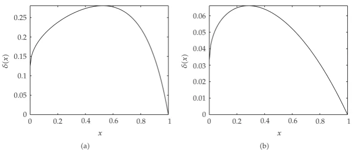
x b Figure 1:δxforαβ1aand forα5,β0.5b.
The approximation foruis a collocation function
pt:pit, t∈τi, τi1, i0, . . . , N−1, 3.4
where we requirep∈Cq−10,1in case that the order of the underlying differential equation
isq. Here,piare polynomials of maximal degreem−1qwhich satisfy the system3.2aat
minnercollocation points
#
ti,j τiρjτi1−τi, i0, . . . , N−1, j1, . . . , m
$
, 0< ρ1<· · ·< ρm<1, 3.5
and the associated boundary conditions3.2b.
Classical theory, compare18, predicts that the convergence order for the global error
of the method is at leastOhm, where his the maximal stepsize, h : max
iτi1 −τi. To
increase efficiency, an adaptive mesh selection strategy based on an a posteriori estimate for
the global error of the collocation solution is utilized. A more detailed description of the
numerical approach can be found in4.
The codebvpsuitealso allows to follow a path in the parameter-solution space. This
means that in the following problem setting, parameterϑis unknown:
F!t, u4t, u3t, ut, ut, ut, ϑ"0, 0≤t≤1, 3.6a
b!u30, u0, u0, u0, u31, u1, u1, u1"0, ϑλ, 3.6b
whereλis given. The path following strategy can also cope with turning points in the path.
The theoretical justification for the path following strategy implemented in bvpsuitehas
been given in19.
We first study the boundary problem 1.9a-1.9b. Positive solutions of problem
The above analytical discussion indicates that depending on the values ofα,β,λ, the problem has one or more positive solutions, a pseudo dead core solution or a dead core
solution. All numerical approximations have been calculated on a fixed mesh withN 500
subintervals and collocation degreem4.Figure 1showsδxfor our choice of parameters
used in the following sections. Here,δis given by2.81.
3.1. Positive Solutions
Forλ ∈ 0, δ0,δ0 4/93/3α4β3/2, there exist a unique positive solution. This
solution was found numerically by using the original problem formulation1.9a-1.9b. For
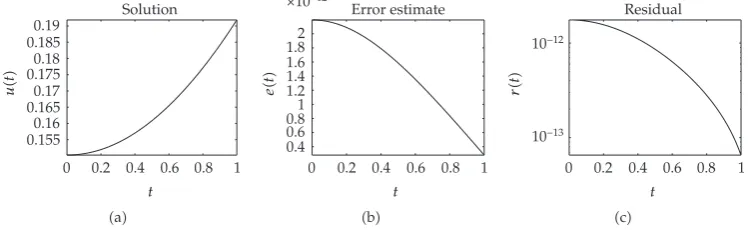
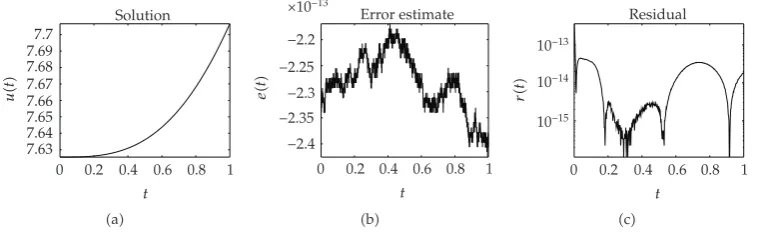
αβ1 we obtainδ0≈0.12469. InFigure 2we display the numerical solution, the error
estimate and the residual for λ 0.05. The residualrt is calculated by substituting the
numerical solutionptinto the differential equation,
rt:pt−λ
pt. 3.7
Due to the very small size of the error estimate and residual, it is obvious that the numerical approximation is very accurate. According to the analytical results, a solution to
the problem satisfies|u0−x0u1|0 wherex0is a root ofδx−λ0. Here, we havex0
0.972608 and|u0−x0u1|6.4 10−8 which again shows the high quality of the numerical
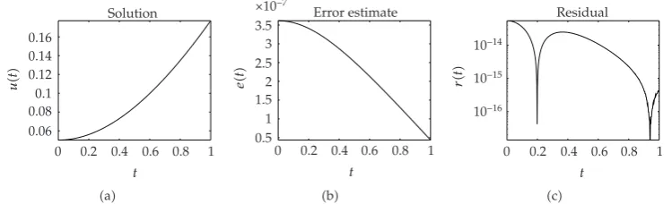
solution. InFigure 3we depict the results for the parameterα 5,β 0.5 andλ 0.02 <
δ0≈0.03294. For this choice of parametersx00.877692 and|u0−x0u1|3.5 10−8.
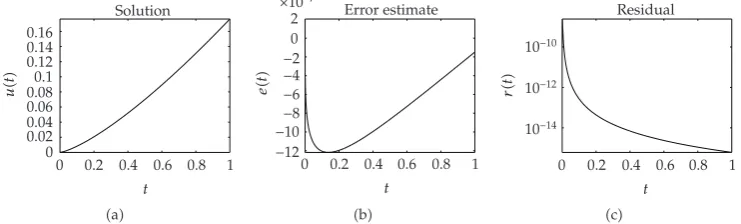
Forλδ0 4/93/3α4β3/2there exists a unique positive solution. To compute
its numerical approximation, we rewrite the problem1.9a-1.9band consider
ut
ut λ 4
9 3
3α4β
3/2
, t∈0,1,
u0 0, αu1 βu1 1, α >0, β >0.
3.8
The numerical results related to parameter setsα1,β1, andα5,β0.5 are shown in
Figure 4andFigure 5, respectively.
Again, the error estimate and the residual are both very small andx0 0.919315, so
|u0−x0u1| 3.5 10−7. Moreover, for the second set of parameters, x0 0.783283 and
|u0−x0u1|1.7 10−8.
Forλ ∈δ0, MwithMmax{δx: 0≤x≤1}there exist two positive solutions.
These two different solutions for a fixed value ofλcan be characterized via the rootsx1,2 of
δx−λ 0 for x ∈ 0,1. The choice of parameters remains the same. Forα 1, β 1
andλ0.15 the solution corresponding tox1 ≈0.009159 is shown inFigure 6. The solution
corresponding tox2 ≈0.896054 is depicted inFigure 7. Note that for these values ofαandβ
0.925
Figure 3:Problem1.9a-1.9b: The numerical solution, the error estimate, and the residual forα 5,
β0.5 andλ0.02.
Figure 4:Problem3.8: The numerical solution, the error estimate, and the residual forα1,β1 and
0.05
Figure 6:Problem3.8: The numerical solution, the error estimate, and the residual forα1,β1 and
λ0.15. The associated root isx1.
Figure 7:Problem3.9: The numerical solution, the error estimate, and the residual forα1,β1 and
0.3
Figure 10:Problem3.8: The numerical solution, the error estimate, and the residual forα1,β1 and
λ0.28049410745840.
0.06
λ0.06608546529011.
The first of those two solutions was found using the reformulated problem3.8withλ
as the right-hand side. For the second solution it was necessary to rewrite the problem again and use
withxas a free unknown parameter andxx2as a necessary additional boundary condition.
Here,x10.009159 and|u0−x1u1|1.7 10−15. For comparison,x20.896054 and|u0−
0
Figure 12:Problem3.10: The numerical solution, the error estimate, and the residual forα1,β1 and
λ 4/93/3α4β3/2.
3.2. Pseudo Dead Core Solutions
In order to calculate the pseudo dead core solutions, we solved the following problem:
ut
utut λut, t∈0,1,
u0 0, αu1 βu1 1, α >0, β >0,
3.10
where the differential equation has been premultiplied by the factor u. Otherwise, the
problem formulated as 3.1 or3.8, would have not been well defined at all pointst /0
such thatut 0. In Figures12and13, we report on the pseudo dead core solutions for
λ 4
In this case, the analytical unique pseudo dead core solution is known,
ut 3
3α4βt
0 0.05 0.1 0.15 0.2
u0
t
Initial profile
0 0.2 0.4 0.6 0.8 1
t a
0 0.05 0.1 0.15 0.2 0.25 0.3 0.35
u
t
Solution
0 0.2 0.4 0.6 0.8 1
t b
−15
−10
−5 0
×10−6
e
t
Error estimate
0 0.2 0.4 0.6 0.8 1
t c
10−60 10−40 10−20
r
t
Residual
0 0.2 0.4 0.6 0.8 1
t d
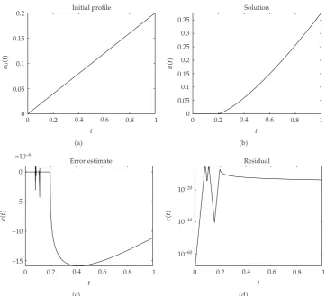
Figure 14:Problem3.10: The initial profile, the numerical solution, the error estimate, and the residual forα1,β1 andt10.2.
Table 1:Problem3.10: Exact global error of the pseudo dead core solution.
α β maxt∈0,1|ut−pt|
1 1 1.5·10−5
5 0.5 5.1·10−6
Therefore, the exact global error is accessible. InTable 1, we show the values for the global
error, max0≤t≤1|ut−pt|whereptis the numerical solution att.
3.3. Dead Core Solutions
We now deal with the dead core solutions of the problem. Note that they only occur for
λ > 4
9 3
3α4β
3/2
0 0.05 0.1 0.15 0.2
u0
t
Initial profile
0 0.2 0.4 0.6 0.8 1
t a
0 0.02 0.04 0.06 0.08 0.1 0.12
u
t
Solution
0 0.2 0.4 0.6 0.8 1
t b
−2
−1.5
−1
−0.5 0
×10−5
e
t
Error estimate
0 0.2 0.4 0.6 0.8 1
t c
10−200 10−100
r
t
Residual
0 0.2 0.4 0.6 0.8 1
t d
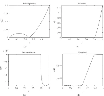
Figure 15:Problem3.10: The initial profile, the numerical solution, the error estimate, and the residual forα1,β1 andt10.8.
Moreover, the relation betweenλandt1, wheret1is such that the solution vanishes on0, t1,
is given by
λ 4
91−t1
3
3α1−t1 4β
3/2
. 3.14
Also, the dead core solution is known,
ut 3
2
λt−t1
4/3
, t∈t1,1. 3.15
For the experiments, we usedt10.2 andt10.8, in order to solve the problem,
ut
utut λut, t∈t1,1,
ut1 0, αu1 βu1 1, α >0, β >0.
0 0.1 0.2 0.3 0.4 0.5 0.6 0.7 0.8
u0
t
Initial profile
0 0.2 0.4 0.6 0.8 1
t a
0 0.02 0.04 0.06 0.08 0.1 0.12 0.14 0.16
u
t
Solution
0 0.2 0.4 0.6 0.8 1
t b
−4
−3
−2
−1 0
×10−6
e
t
Error estimate
0 0.2 0.4 0.6 0.8 1
t c
10−80 10−60 10−40 10−20
r
t
Residual
0 0.2 0.4 0.6 0.8 1
t d
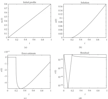
Figure 16:Problem3.10: The initial profile, the numerical solution, the error estimate, and the residual forα5,β0.5 andt10.2.
Clearly, if we approached the problem3.16 directly, we had to use the knowledge of t1
which is not available in general. Therefore, it is especially important to note that we were
able to find the dead core solution without explicit knowledge oft1by treating the problem
3.10, formulated on the whole interval0,1,
ut
utut λut, t∈0,1,
u0 0, αu1 βu1 1, α >0, β >0,
3.17
instead of solving3.16. In Figures14and15, we report on the numerical test runs forα1,
β1, and two values oft1,t10.2 andt10.8, respectively. In Figures16and17, analogous
0 0.05 0.1 0.15 0.2
u0
t
Initial profile
0 0.2 0.4 0.6 0.8 1
t a
0 0.02 0.04 0.06 0.08 0.1 0.12
u
t
Solution
0 0.2 0.4 0.6 0.8 1
t b
−16
−14
−12
−10
−8
−6
−4
−2 0
×10−6
e
t
Error estimate
0 0.2 0.4 0.6 0.8 1
t c
10−300 10−200 10−100
r
t
Residual
0 0.2 0.4 0.6 0.8 1
t d
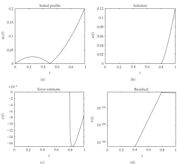
Figure 17:Problem3.10: The initial profile, the numerical solution, the error estimate, and the residual forα5,β0.5 andt10.8.
Table 2 contains the information on the exact global error of the numerical dead
core solution. We report on its maximal value maxt∈0,1|ut− pt| for a wide range of
parameters. Obviously, dead core solutions can be found without exact use of the known solution structure, but the initial profile must be chosen carefully to guarantee the Newton iteration to convergence.
3.4. Positive Solutions of Problem
1.5a
-
1.5b
In this section, we deal with problem1.5a-1.5b. Since this problem is very involved, we
decided to simulate it numerically first in order to provide some preliminary information
about its solution. The numerical treatment of 1.5a-1.5b turned out to be not at all
straightforward, but nevertheless, for a certain choice of parameters, γ 3, ρ 2, ν 2,