METHODS FOR DETERMINATION AND APPROXIMATION
OF THE DOMAIN OF ATTRACTION IN THE CASE OF
AUTONOMOUS DISCRETE DYNAMICAL SYSTEMS
ST. BALINT, E. KASLIK, A. M. BALINT, AND A. GRIGISReceived 15 October 2004; Accepted 18 October 2004
A method for determination and two methods for approximation of the domain of attrac-tionDa(0) of the asymptotically stable zero steady state of an autonomous,R-analytical, discrete dynamical system are presented. The method of determination is based on the construction of a Lyapunov functionV, whose domain of analyticity isDa(0). The first method of approximation uses a sequence of Lyapunov functionsVp, which converge to the Lyapunov functionVonDa(0). EachVpdefines an estimateNpofDa(0). For anyx∈ Da(0), there exists an estimateNpxwhich containsx. The second method of approxima-tion uses a ballB(R)⊂Da(0) which generates the sequence of estimatesMp=f−p(B(R)). For anyx∈Da(0), there exists an estimateMpxwhich containsx. The cases∂0f<1 and ρ(∂0f)<1≤ ∂0fare treated separately because significant differences occur.
Copyright © 2006 Hindawi Publishing Corporation. All rights reserved.
1. Introduction
Let be the following discrete dynamical system:
xk+1=f
xk k=0, 1, 2,..., (1.1)
where f :Ω→Ωis an R-analytic function defined on a domain Ω⊂Rn, 0∈Ωand f(0)=0, that is,x=0 is a steady state (fixed point) of (1.1).
Forr >0, denote byB(r)= {x∈Rn:x< r}the ball of radiusr.
The steady statex=0 of (1.1) is “stable” provided that given any ballB(ε), there is a ballB(δ) such that ifx∈B(δ) then fk(x)∈B(ε), fork=0, 1, 2,...[4].
If in addition there is a ballB(r) such thatfk(x)→0 ask→ ∞for allx∈B(r) then the steady statex=0 is “asymptotically stable” [4].
The domain of attractionDa(0) of the asymptotically stable steady statex=0 is the set of initial statesx∈Ωfrom which the system converges to the steady state itself, that is,
Da(0)=x∈Ω|fk(x)−−−→k→∞ 0. (1.2)
Hindawi Publishing Corporation Advances in Difference Equations Volume 2006, Article ID 23939, Pages1–15
Theoretical research shows that theDa(0) and its boundary are complicated sets [5–9]. In most cases, they do not admit an explicit elementary representation. The domain of attraction of an asymptotically stable steady state of a discrete dynamical system is not necessarily connected (which is the case for continuous dynamical systems). This fact is shown by the following example.
Example 1.1. Let be the functionf :R→Rdefined byf(x)=(1/2)x−(1/4)x2+ (1/2)x3+ (1/4)x4. The domain of attraction of the asymptotically stable steady statex=0 isDa(0)= (−2.79,−2.46)∪(−1, 1) which is not connected.
Different procedures are used for the approximation of theDa(0) with domains hav-ing a simpler shape. For example, in the case of [4, Theorem 4.20, page 170] the domain which approximates theDa(0) is defined by a Lyapunov functionV built with the ma-trix∂0f of the linearized system in 0, under the assumption∂0f<1. In [2], a Lya-punov function V is presented in the case when the matrix∂0f is a contraction, that is,∂0f<1. The Lyapunov functionV is built using the whole nonlinear system, not only the matrix∂0f.V is defined on the wholeDa(0), and more, theDa(0) is the nat-ural domain of analyticity ofV. In [3], this result is extended for the more general case whenρ(∂0f)<1 (whereρ(∂0f) denotes the spectral radius of∂0f.) This last result is the following.
Theorem1.2 (see [3]). If the function f satisfies the following conditions:
f(0)=0, ρ∂0f
<1, (1.3)
then0is an asymptotically stable steady state.Da(0)is an open subset ofΩand coincides with the natural domain of analyticity of the unique solutionV of the iterative first-order functional equation
Vf(x)−V(x)= −x2,
V(0)=0. (1.4)
The functionV is positive onDa(0)andV(x)x→→x0+∞, for anyx0∈∂Da(0), (∂Da(0) de-notes the boundary ofDa(0)) or forx → ∞.
The functionV is given by
V(x)= ∞
k=0
fk(x)2
for anyx∈Da(0). (1.5)
The Lyapunov functionV can be found theoretically using relation (1.5). In the fol-lowings, we will shortly present the procedure of determination and approximation of the domain of attraction using the functionV presented in [2,3].
The region of convergenceD0of the power series development ofVin 0 is a part of the domain of attractionDa(0). IfD0is strictly contained inDa(0), then there exists a point x0∈∂D
series development ofVinx0. The domain of convergenceD
1of the series centered inx0 gives a new partD1\(D0D1) of the domain of attractionDa(0). At this step, the part D0 D1ofDa(0) is obtained.
If there exists a pointx1∈∂(D
0 D1) such that the functionVis bounded on a neigh-borhood ofx1, then the domainD
0 D1is strictly included in the domain of attraction Da(0). In this case, the procedure described above is repeated inx1.
The procedure cannot be continued in the case when it is found that on the boundary of the domainD0 D1 ··· Dp obtained at stepp, there are no points having neigh-borhoods on whichV is bounded.
This procedure gives an open connected estimateDof the domain of attractionDa(0). Note that f−k(D),k∈Nis also an estimate ofDa(0), which is not necessarily connected.
The procedure described above is illustrated by the following examples.
Example 1.3. Let be the f :R→Rdefined by f(x)=x2. Due to the equalityfk(x)=x2k the domain of attraction of the asymptotically stable steady statex=0 isDa(0)=(−1, 1). The Lyapunov function isV(x)=∞k=0x2
k+1
. The domain of convergence of the series is D0=(−1, 1) which coincides withDa(0).
The radius of convergence of the series (1.6) is
r0=mlim→∞m
therefore the domain of convergence of the power series development ofVin−1 isD−1= (−2, 0) which gives a new part ofDa(0).
2. Theoretical results when the matrixA=∂0f is a contraction (i.e.,A<1) The function f can be written as
f(x)=Ax+g(x) for anyx∈Ω, (2.1)
whereA=∂0f andg:Ω→Ωis anR-analytic function such thatg(0)=0 and limx→0(g(x)
/x)=0.
Proposition2.1. IfA<1, then there existsr >0such thatB(r)⊂Ωandf(x)<x
for anyx∈B(r)\ {0}.
Proof. Due to the fact that limx→0(g(x)/x)=0 there existsr >0 such thatB(r)⊂Ω
and
g(x)<
1− Ax for anyx∈B(r)\ {0}. (2.2)
Let bex∈B(r)\ {0}. Inequality (2.2) provides that
f(x)=Ax+g(x)≤ Ax+g(x)<
A+ 1− Ax = x (2.3)
therefore,f(x)<x.
Definition 2.2. LetR >0 be the largest number such thatB(R)⊂Ωandf(x)<xfor anyx∈B(R)\ {0}.
If for anyr >0,B(r)⊂Ωandf(x)<xfor anyx∈B(r)\ {0}, thenR=+∞and B(R)=Ω=Rn.
Lemma2.3. (a)B(R)is invariant to the flow of system (1.1).
(b)For anyx∈B(R), the sequence(fk(x))
k∈Nis decreasing.
(c)For anyp≥0andx∈B(R)\ {0},ΔVp(x)=Vp(f(x))−Vp(x)<0, where
Vp(x)= p
k=0
fk(x)2
for x∈Ω. (2.4)
Proof. (a) Ifx=0, then fk(0)=0, for anyk∈N. Forx∈B(R)\ {0}, we havef(x)<
x, which implies thatf(x)∈B(R), that is,B(R) is invariant to the flow of system (1.1). (b) By induction, it results that forx∈B(R) we have fk(x)∈B(R) andfk+1(x) ≤
fk(x), which means that the sequence (fk(x))k
∈Nis decreasing.
(c) In particular, for p≥0 and x∈B(R), we have fp+1(x) ≤ f(x)<x and therefore,ΔVp(x)= fp+1(x)2− x2<0.
Corollary2.4. For anyp≥0, there exists a maximal domainGp⊂Ωsuch that0∈Gp
and forx∈Gp\ {0}, the (positive definite) functionVpverifiesΔVp(x)<0. In other words, for any p≥0, the function Vp defined by (2.4) is a Lyapunov function for (1.1) onGp. Moreover,B(R)⊂Gpfor anyp≥0.
Theorem2.5. B(R)is an invariant set included in the domain of attractionDa(0).
The sequence (fk(x))k∈Nis bounded: fk(x) belongs toB(R). Let be (fkj(x))j∈Na
con-vergent subsequence and let be limj→∞fkj(x)=y0. It is clear thaty0∈B(R).
It can be shown that
fk(x)≥y0 for anyk∈N. (2.5)
For this, observe first that fkj(x)→y0 and (fkj(x))k
∈N is decreasing (Lemma 2.3).
These imply thatfkj(x) ≥ y0for anykj. On the other hand, for anyk∈N, there exists kj∈N such that kj≥k. Therefore, as the sequence (fk(x))
k∈N is decreasing
(Lemma 2.3), we obtain thatfk(x) ≥ fkj(x) ≥ y0.
We show now thaty0=0. Suppose the contrary, that is,y0=0. Inequality (2.5) becomes
fk(x)≥y0>0 for anyk∈N. (2.6)
By means ofLemma 2.3, we have thatf(y0)<y0.
Therefore, there exists a neighborhoodUf(y0)⊂B(R) of f(y0) such that for anyz∈
Uf(y0) we havez<y0. On the other hand, for the neighborhoodUf(y0) there
ex-ists a neighborhoodUy0⊂B(R) of y0such that for any y∈Uy0, we have f(y)∈Uf(y0).
Therefore:
f(y)<y0 for anyy∈Uy0. (2.7)
As fkj(x)→y0, there exists ¯jsuch that fkj(x)∈Uy0, for any j≥j¯. Makingy= fkj(x) in (2.7), it results that
fkj+1(x)=ffkj(x)<y0 for j≥j¯ (2.8)
which contradicts (2.6). This means thaty0=0, consequently, every convergent subse-quence of (fk(x))k∈Nconverges to 0. This provides that the sequence (fk(x))k∈Nis
con-vergent to 0, andx∈Da(0).
Therefore, the ballB(R) is contained in the domain of attraction ofDa(0). Forp≥0 andc >0 let beNpcthe set
Nc
p=x∈Ω:Vp(x)< c. (2.9)
Ifc=+∞, thenNcp=Ω.
Theorem2.6. Let bep≥0. For anyc∈(0, (p+ 1)R2], the setNc
pis included in the domain of attractionDa(0).
Proof. Let bec∈(0, (p+ 1)R2] andx∈Nc
p. ThenVp(x)=kp=0fk(x)2< c≤(p+ 1)R2, therefore, there exists k∈ {0, 1,...,p}such thatfk(x)2< R2. It results that fk(x)∈
B(R)⊂Da(0), therefore,x∈Da(0).
cp=(p+ 1)R2. In the followings, we will use the notation Np instead ofNcp
p . Shortly, Np= {x∈Ω:Vp(x)<(p+ 1)R2}is a part ofDa(0). Let us note thatN
0=B(R).
Remark 2.8. IfR=+∞(i.e.,Ω=Rnandf(x)<x, for anyx∈R\ {0}), thenNp=
Rnfor anyp≥0 andDa(0)=Rn.
Theorem2.9. For the sets(Np)p∈N, the following properties hold:
(a)for anyp≥0, one hasNp⊂Np+1; (b)for anyp≥0, the setNpis invariant to f;
(c)for anyx∈Da(0), there existspx≥0such thatx∈Npx.
Proof. (a) Let bep≥0 andx∈Np. ThenVp(x)=kp=0fk(x)2<(p+ 1)R2, therefore, there exists k∈ {0, 1,...,p}such that fk(x)2< R2. It results that fk(x)∈B(R) and therefore fm(x)∈B(R), for anym≥k. Form=p+ 1 we obtainfp+1(x)< R, hence Vp+1(x)=Vp(x) +fp+1(x)2<(p+ 1)R2+R2=(p+ 2)R2. Therefore,x∈Np+1.
(b) Let be x∈Np. If x< R then fm(x)< R for any m≥0 (by means of
Lemma 2.3). This implies that Vp(f(x))=kp=0fk(f(x))2=
p+1
k=1fk(x)2<(p+ 1)R2, meaning that f(x)∈Np.
Let us suppose thatx ≥R. Asx∈Np, we have thatVp(x)=pk=0fk(x)2<(p+ 1)R2, therefore, there existsk∈ {0, 1,...,p}such thatfk(x)< R. It results that fk(x)∈ B(R) and thereforefm(x)∈B(R), for anym≥k. Form=p+ 1 we obtainfp+1(x)< R. This implies that
Vpf(x)=Vp(x) +fp+1(x)2− x2<(p+ 1)R2+R2−R2=(p+ 1)R2 (2.10)
therefore f(x)∈Np.
(c) Suppose the contrary, that is, there existx∈Da(0) such that for any p≥0,x /∈
Np. Therefore,Vp(x)≥(p+ 1)R2 for any p≥0. Passing to the limit for p→ ∞in this inequality, provides thatV(x)= ∞. This means x∈∂Da(0) which contradicts the fact that x belongs to the open setDa(0). In conclusion, there exists px≥0 such that x∈
Npx.
Forp≥0 let beMp= f−p(B(R))= {x∈Ω: fp(x)∈B(R)}, obtained by the trajectory reversing method.
Theorem2.10. The following properties hold:
(a)Mp⊂Da(0)for anyp≥0; (b)for anyp≥0,Mpis invariant to f;
(c)Mp⊂Mp+1for anyp≥0;
(d)for anyx∈Da(0), there existspx≥0such thatx∈Mpx.
Proof. (a) AsMp=f−p(B(R)) andB(R)⊂Da(0) (seeTheorem 2.5) it is clear thatMp⊂ Da(0).
(b) and (c) follow easily by induction, usingLemma 2.3.
Both sequences of sets (Mp)p∈Nand (Np)p∈Nare increasing, and are made up of
esti-mates ofDa(0). From the practical point of view, it is important to know which sequence converges more quickly. The next theorem provides that the sequence (Mp)p∈Nconverges
more quickly than (Np)p∈N, meaning that for p≥0, the setMp is a larger estimate of
3. Theoretical results whenA=∂0f is a convergent noncontractive matrix (i.e.,ρ(A)<1≤ A)
The formula of variation of constants for anypgives:
If for anyr >0, we have thatB(r)⊂Ωandfp(x)<xfor any p∈ {p,p+ 1,..., 2p−1}andx∈B(r)\ {0}, thenR=+∞andB(R)=Ω=Rn.
Lemma3.3. (a)For anyx∈B(R)andp∈{p,p+ 1,..., 2p−1}, the sequence(fkp(x))k
∈N
is decreasing.
(b)For anyp≥pandx∈B(R)\ {0},fp(x)<x.
(c)For any p≥pandx∈B(R)\ {0},ΔVp(x)=Vp(f(x))−Vp(x)<0, where Vp is defined by (2.4).
Proof. (a) Ifx=0, then fp(0)=0, for anyp≥0.
Let bex∈B(R)\ {0}. We know thatfp(x)<xfor anyp∈ {p,p+ 1,..., 2p−1}. It results that fp(x)∈B(R) for anyp∈ {p,p+ 1,..., 2p−1}. This implies that for any k∈Nwe havefkp(x)<xandf(k+1)p(x) ≤ fkp(x), meaning that the sequence (fkp(x))
k∈Nis decreasing.
(b) Let bex∈B(R)\ {0}. Inequalityfp(x)<xis true for any p∈ {p,p+ 1,..., 2p−1}.
Let bep≥2p. There existsq∈Nand p∈ {p,p+ 1,..., 2p−1}such thatp=qp+
p. Using (a), we have that fp
(x)∈B(R) and fqp(y)≤ y, for anyy∈B(R), therefore
fp(x)=fqpfp
(x)≤fp
(x)<x (3.4)
(c) results directly from (b).
Corollary3.4. For anyp≥p, there exists a maximal domainGp⊂Ωsuch that0∈Gp
and for anyx∈Gp\ {0}, the (positive definite) functionVp verifiesΔVp(x)<0. In other words, for anyp≥p, the functionVpis a Lyapunov function for (1.1) onGp. More,B(R)⊂ Gpfor anyp≥p.
Lemma3.5. For anyk≥p, there existsqk∈Nsuch that
f(qk+3)p(x)≤fk(x)≤fqkp(x) for anyx∈B R. (3.5)
Proof. Let bek≥p. There exists a uniqueqk∈Nand a uniquepk∈ {p,p+ 1,..., 2p−1}
such thatk=qkp+pk.Lemma 3.3provides that for anyx∈B(R) we have thatfqkp(x)∈ B(R) andfpk(x) ≤ x. It results that
fk(x)=fpkfqkp(x)≤fqkp(x) for anyx∈BR¯. (3.6)
On the other hand, we have (qk+ 3)p=k+ (3p−pk). As (3p−pk)∈ {p+ 1,p+ 2,..., 2p}
f3p−pk(x) ≤ x. Therefore
f(qk+3)p(x)=f3p−pkfk(x)≤fk(x) for anyx∈B R. (3.7)
Combining the two inequalities, we get that
f(qk+3)p(x)≤fk(x)≤fqkp(x) for anyx∈B R (3.8)
which concludes the proof.
Theorem3.6. B(R)is included in the domain of attractionDa(0).
Proof. Let bex∈B(R)\ {0}. We have to prove that limk→∞fk(x)=0.
The sequence (fk(x))k∈Nis bounded (seeLemma 3.3). Let be (fkj(x))j∈Na convergent
subsequence and let be limj→∞fkj(x)=y0.
We suppose, without loss of generality, thatkj≥pfor any j∈N.Lemma 3.5provides that for anyj∈Nthere existsqj∈Nsuch that
f(qj+3)p(x)≤fkj(x)≤fqjp(x). (3.9)
As (fqjp(x))j
∈Nand (f(qj+3)p(x))j∈N are subsequences of the convergent sequence
(fqp(x))q
∈N(decreasing, according toLemma 3.3), it results that they are convergent.
The double inequality (3.9) provides that limj→∞fqjp(x) = y0. Therefore, limq→∞ fqp(x) = y0.
It can be shown that
fk(x)≥y0 for anyk≥p. (3.10)
For this, remark that limq→∞fqp(x) = y0and (fqp(x))q∈Nis decreasing (Lemma 3.3), which implies thatfqp(x) ≥ y0for anyq∈N. On the other hand,Lemma 3.5 provides that for anyk≥pthere existsqksuch thatf(qk+3)p(x) ≤ fk(x). Therefore,
fk(x) ≥ f(qk+3)p(x) ≥ y0, for anyk≥p.
We show now thaty0=0. Suppose the contrary, that is,y0=0. Inequality (3.10) becomes
fk(x)≥y0>0 for anyk≥p. (3.11)
By means ofLemma 3.3, we have thatfp(y0)<y0.
There exists a neighborhoodUfp(y0)⊂B(R) of fp(y0) such that for anyz∈Ufp(y0)we
havez<y0. On the other hand, for the neighborhoodU
fp(y0)there exists a
neigh-borhoodUy0⊂B(R) ofy0such that for anyy∈Uy0, we havefp(y)∈Ufp(y0). Therefore:
As fkj(x)→y0, there exists ¯jsuch that fkj(x)∈Uy0, for any j≥j¯. Makingy= fkj(x) in (3.12), it results that
fkj+p(x)=fpfkj(x)<y0 for j≥j¯ (3.13)
which contradicts (3.11). This means that y0=0, consequently, every convergent sub-sequence of (fk(x))k∈N converges to 0. This provides that the sequence (fk(x))k∈N is
convergent to 0, andx∈Da(0).
Therefore, the ballB(R) is contained in the domain of attraction ofDa(0).
Theorem3.7. Let bep≥0. For anyc∈(0, (p+ 1)R2], the setNc
pis included in the domain of attractionDa(0).
Proof. Let bec∈(0, (p+ 1)R2] andx∈Nc
p. ThenVp(x)=kp=0fk(x)2< c≤(p+ 1)R2, therefore, there exists k∈ {0, 1,...,p}such thatfk(x)2<R2. It results that fk(x)∈
B(R)⊂Da(0), therefore,x∈Da(0).
Remark 3.8. It is obvious that forp≥0 and 0< c< cone hasNpc⊂Npc. Therefore, for a givenp≥0, the largest part ofDa(0) which can be found by this method isNpcp, where
cp=(p+ 1)R2. In the followings, we will use the notation Np instead ofNcp
p . Shortly,
Np= {x∈Ω:Vp(x)<(p+ 1)R2}is a part ofDa(0). Let us note thatN
0=B(R).
Remark 3.9. IfR=+∞(i.e.,Ω=Rnandfp(x)<x, for anyp∈ {p,p+ 1,..., 2p−1} andx∈R\ {0}), thenNp =Rnfor anyp≥0 andDa(0)=Rn.
Theorem3.10. For anyx∈Da(0)there existspx≥0such thatx∈Np x.
Proof. Let bex∈Da(0). Suppose the contrary, that is,x /∈Np for any p≥0. Therefore, Vp(x)≥(p+ 1)R2for anyp≥0. Passing to the limit when p→ ∞in this inequality pro-vides thatV(x)= ∞. This meansx∈∂Da(0) which contradicts the fact thatxbelongs to the open setDa(0). In conclusion, there existspx≥0 such thatx∈Np x. Remark 3.11. The sequence of sets (Np )p∈N is generally not increasing (seeSection 4:
Numerical examples, the Van der Pol equation).
Open question. Is the sequence of sets (Np )p≥pincreasing?
Forp≥0 let beMp = f−p(B(R))= {x∈Ω: fp(x)∈B(R)}, obtained by the trajectory reversing method.
Theorem3.12. For the sets(Mp)p∈N, the following properties hold:
(a)Mp ⊂Da(0), for anyp≥0;
(b)Mkp ⊂M(k+1)pfor anyk∈Nandp∈ {p,p+ 1,..., 2p−1}; (c)for anyx∈Da(0), there existspx≥0such thatx∈Mpx.
Proof. (a) AsMp=f−p(B(R)) andB(R)⊂Da(0) (seeTheorem 3.6) it is clear thatMp ⊂ Da(0).
(b) follows easily by induction, usingLemma 3.3.
−1 0.5
0 −0.5
−1 −1 −0.5 0 0.5 1
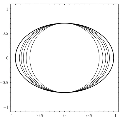
Figure 4.1. The setsNp,p=0, 4 and∂Da(0, 0) for (4.1).
Remark 3.13. The sequence of sets (Mp )p∈N is generally not increasing (seeSection 4:
Numerical examples, the Van der Pol equation).
Both sequences of sets (Mp )p∈Nand (Np )p∈Nare made up of estimates ofDa(0). From
the practical point of view, it would be important to know which one of the setsMp or
Npis a larger estimate ofDa(0) for a fixedp≥p. Such result could not be established, but the following theorem holds.
Theorem3.14. For anyp≥0, one hasNp ⊂Mp+p.
Proof. Let bep≥0 andx∈Np . We have thatVp(x)=kp=0fk(x)2<(p+ 1)R2, there-fore, there existsk∈ {0, 1,...,p}such thatfk(x)<R. This implies thatfk+m(x)∈B(R), for anym≥p. Form=p−k+pwe obtain fp+p(x)∈B(R), meaning thatx∈Mp
+p.
4. Numerical examples
4.1. Example with known domain of attraction. Let the following discrete dynamical system be
xk+1=1 2xk
1 +x2 k+ 2y2k yk+1=1
2yk
1 +x2k+ 2yk2
k∈N. (4.1)
−1 0.5
0 −0.5
−1 −1 −0.5 0 0.5 1
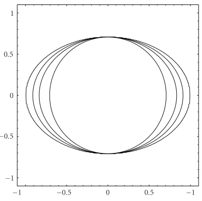
Figure 4.2. The setsMp,p=0, 1, 2, 6 for (4.1).
As∂(0,0)f =1/2, we compute the largest numberR >0 such thatf(x)<xfor anyx∈B(R)\ {0}, and we findR=0.7071.
For p=0, 1, 2, 3, 4, we find theNp sets shown inFigure 4.1, parts ofDa(0, 0) (Np⊂
Np+1, for p≥0). InFigure 4.1, the thick-contoured ellipsis represents the boundary of Da(0, 0).
InFigure 4.2, the sets Mp are represented, for p=0, 1, 2, 6 (Mp⊂Mp+1, for p≥0). Note thatM6approximates with a good accuracy the domain of attraction.
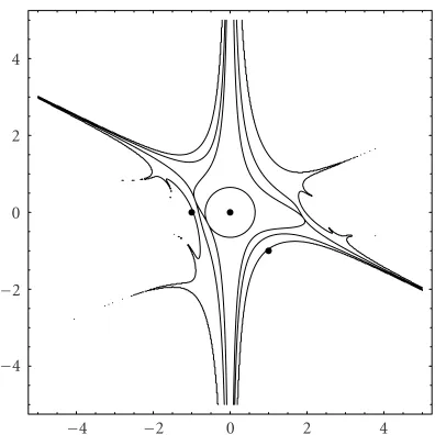
4.2. Discrete predator-prey system. We consider the discrete predator-prey system:
xk+1=axk
1−xk−xkyk
yk+1=1bxkyk
witha=1
2,b=1,k∈N. (4.2)
The steady states of this system are (0, 0) (asymptotically stable), (−1, 0) and (1,−1) (both unstable).
We have that∂(0,0)f =1/2, and the largest numberR >0 such thatf(x)<xfor anyx∈B(R)\ {0}isR=0.65.
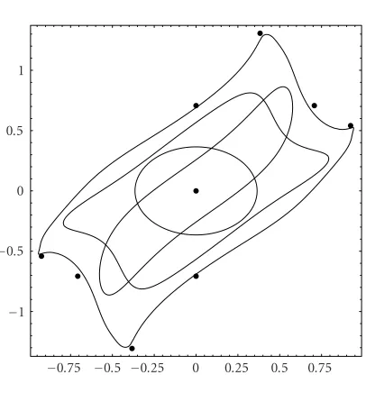
Figure 4.3presents theNpsets for p=0, 1, 2, 3, 4, 5, parts ofDa(0, 0) (Np⊂Np+1, for p≥0). The black points inFigure 4.3represent the steady states of the system.
1.5 1
0.5 0
−0.5 −1
−1.5 −1 −0.5 0 0.5 1 1.5
Figure 4.3. The setsNp,p=0, 5 for (4.2).
4 2
0 −2 −4
−4 −2 0 2 4
Figure 4.4. The setsMp,p=0, 1, 2, 6 for (4.2).
4.3. Discrete Van der Pol system. Let the following discrete dynamical system, obtained from the continuous Van der Pol system be
xk+1=xk−yk
0.75 0.5 0.25 0 −0.25 −0.5 −0.75 −1 −0.5 0 0.5 1
Figure 4.5. The setsNp,p=0, 5 for (4.3).
0.75 0.5 0.25 0 −0.25 −0.5 −0.75 −1 −0.5 0 0.5 1
Figure 4.6. The setsMp,p=0, 1, 2, 6 for (4.3).
The only steady state of this system is (0, 0) which is asymptotically stable. There are many periodic points for this system, the periodic points of order 2, 5 being represented inFigure 4.5by the black points.
The largest number R > 0 such that fp(x)<x for p∈ {p,p+ 1,..., 2p−1} =
{2, 3}andx∈B(R)\ {0}isR=0.365.
Forp=0, 1, 2, 3, 4, 5, the connected components which contain (0, 0) of theNp sets are shown inFigure 4.5. We have thatN0N1⊂N2⊂N3⊂N4⊂N5.
InFigure 4.6, the setsMp are represented, for p=0, 1, 2, 6. Note that the inclusions
Mp⊂Mp+1do not hold.
References
[1] R. A. Horn and C. R. Johnson,Matrix Analysis, Cambridge University Press, Cambridge, 1985. [2] E. Kaslik, A. M. Balint, S. Birauas, and St. Balint,Approximation of the domain of attraction of an
asymptotically stable fixed point of a first order analytical system of difference equations, Nonlinear Studies10(2003), no. 2, 103–112.
[3] E. Kaslik, A. M. Balint, A. Grigis, and St. Balint,An extension of the characterization of the domain of attraction of an asymptotically stable fixed point in the case of a nonlinear discrete dynamical system, Proceedings of 5th ICNPAA (S. Sivasundaram, ed.), European Conference Publications, Cambridge, UK, 2004.
[4] W. G. Kelley and A. C. Peterson,Difference Equations, 2nd ed., Harcourt/Academic Press, Cali-fornia, 2001.
[5] H. Koc¸ak, Differential and Difference Equations through Computer Experiments, 2nd ed., Springer, New York, 1989.
[6] G. Ladas, C. Qian, P. N. Vlahos, and J. Yan,Stability of solutions of linear nonautonomous diff er-ence equations, Applicable Analysis. An International Journal41(1991), no. 1-4, 183–191. [7] V. Lakshmikantham and D. Trigiante,Theory of Difference Equations. Numerical Methods and
Applications, Mathematics in Science and Engineering, vol. 181, Academic Press, Massachusetts, 1988.
[8] J. P. LaSalle,The Stability and Control of Discrete Processes, Applied Mathematical Sciences, vol. 62, Springer, New York, 1986.
[9] ,Stability theory for difference equations, Studies in Ordinary Differntial Equations (J. Hale, ed.), MAA Studies in Mathematics, vol. 14, Taylor and Francis Science Publishers, London, 1997, pp. 1–31.
St. Balint: Department of Mathematics, West University of Timis¸oara, Bd. V. Parvan 4, 300223 Timis¸oara, Romania
E-mail address:[email protected]
E. Kaslik: Department of Mathematics, West University of Timis¸oara, Bd. V. Parvan 4, 300223 Timis¸oara, Romania
Current address: LAGA, UMR 7539, Institut Galil´ee, Universit´e Paris 13, 99 Avenue J.B. Cl´ement, 93430 Villetaneuse, France
E-mail address:[email protected]
A. M. Balint: Department of Physics, West University of Timis¸oara, Bd. V. Parvan 4, 300223 Timis¸oara, Romania
E-mail address:[email protected]
A. Grigis: LAGA, UMR 7539, Institut Galil´ee, Universit´e Paris 13, 99 Avenue J.B. Cl´ement, 93430 Villetaneuse, France