R E S E A R C H
Open Access
An efficient high-order compact finite
difference scheme based on proper
orthogonal decomposition for the
multi-dimensional parabolic equation
Baozou Xu
1and Xiaohua Zhang
1,2**Correspondence:
1College of Science, China Three
Gorges University, Yichang, China 2Three Gorges Mathematical
Research Center, China Three Gorges University, Yichang, China
Abstract
In this paper, the combination of efficient sixth-order compact finite difference scheme (E-CFDS6) based proper orthogonal decomposition and Strang splitting method (E-CFDS6-SSM) is constructed for the numerical solution of the
multi-dimensional parabolic equation (MDPE). For this purpose, we first develop the CFDS6 to attain a high accuracy for the one-dimensional parabolic equation (ODPE). Then, by the Strang splitting method, we have converted the MDPE into a series of one-dimensional ODPEs successfully, which is easier to implement and program with CFDS6 than an alternating direction implicit method. Finally, we employ proper orthogonal decomposition techniques to improve the computational efficiency of CFDS6 and build the E-CFDS6-SSM with fewer unknowns and sufficiently high accuracy. Six numerical examples are presented to demonstrate that the
E-CFDS6-SSM not only can largely alleviate the computational load but also hold a high accuracy and simplify the process of the program for the numerical solution of MDPE.
Keywords: Compact finite difference scheme; Proper orthogonal decomposition; Multi-dimensional parabolic equation; Strang splitting method
1 Introduction
Many physical phenomena are simulated with parabolic equations such as proliferation of gas, the penetration of liquids, heat conduction and spread of impurities in semicon-ductor materials. However, due to the complexity of practical problems or the lack of rules for initial values, their exact solutions for practical engineering problems are not generally sought out so that we have to rely on numerical solutions. Currently, extensive numeri-cal methods including the finite difference method, finite element method, finite volume method and spectral method have been developed for the numerical solution of parabolic equation. In these methods, the FDM has proved to be the most popular and efficient method for finding the numerical solution of a parabolic equation because of its simplicity, wide application in applied fields of sciences and easy programming. Although it is feasi-ble to solve these equations by means of some traditional FDM such as the Euler method and the central difference method, these schemes, which converge very slowly, may largely
deviate from the exact solution. Therefore, it is imperative for us to construct a scheme that can guarantee satisfying numerical solution and reflect the properties of equations.
In the existing papers, many scholars focus their eyes on the compact finite difference scheme (CFDS), which has been widely used in numerical solution of various types of par-tial differenpar-tial equations. The outstanding advantage of CFDS is that it possesses a faster convergence rate than the corresponding explicit schemes, not significantly increasing the points in each coordinate direction of the grid. As one of the most effective numerical im-plementations, there have been many numerical research reports concerning with CFDS. For example, Hammad [1] constructed CFDS for Burgers–Huxley and Burgers–Fisher equations. Wang [2] developed CFDS for Poisson equation. Mohebbi [3] combined CFDS with a radial basis functions meshless approach to solve the 2D Rayleigh–Stokes problem. Düring [4] applied CFDS to stochastic volatility models on non-uniform grids. Chen [5] provided high-order CFDS to solve parabolic equation. Especially, some attempts have been made whose main idea is to combine fourth Runge–Kutta in time and a sixth-order compact finite difference in space (CFDS6) by the researchers [6–8]. However, the CFDS6 for parabolic equation, especially the case of desirable accuracy in high dimension, they usually need small spatial discretization or extended finite difference stencils and a small time step which brings about heavy computational loads. Therefore, an important prob-lem for CFDS6 is how to build a scheme which not only saves the computational time in the practical problems but also holds a sufficiently accurate numerical solution.
A large number of numerical examples have proved that the proper orthogonal decom-position (POD) is a powerful technique offering the adequate approximation for numerical models with fewer unknowns, which means that the models based on POD can alleviate the computational loads and guarantee sufficiently accurate solution [9–11]. The POD is also known as Karhunen–Loève expansions in signal analysis or principal component analysis in statistics, which has been widely used in real-life applications. Especially, it also has been combined with some numerical methods such as finite element methods [12], meshless methods [13], finite difference methods [14] and finite volume methods [15] suc-cessfully. However, to the best of our knowledge, there are no published results in papers concerning efficient CFDS6 (E-CFDS6) for parabolic equations. Thus, the first task in this paper is to build the E-CFDS6 based on the POD method for the parabolic equations.
main idea is to split the Burgers’ equation into two sub-equations and solve them by fi-nite difference schemes. In [18], the authors have split the full problem into hyperbolic, nonlinear and linear problems, solved by different numerical methods. Sun [19] had ap-plied a splitting method for solving the radiative transfer problem. Therefore, the Strang splitting method (SSM) is an effective numerical method for solving MDPE by convert-ing MDPE to successions of ODPE. Then we just need to solve the sequence of a linear tri-diagonal system, and the whole process of programming is also simplified. SSM has been applied successfully in a diffusion–reaction problem [20]. To the best of our knowl-edge, no high-order CFDS combined with POD and SSM (E-CFDS6-SSM) aimed to solve MDPE efficiently has been developed so far. Hence, the second task in this paper is to de-velop the E-CFDS6-SSM based on the POD and SSM methods to attain a highly accurate numerical solution of MDPE, which only contains very few unknowns and simplifies the whole process of computation.
The outline of this paper is organized as follows. In Sect.2, a brief background is given on the theoretical foundations of high-order compact finite difference scheme and POD tech-nique. Then the formulation of the CFDS6 is given for ODPE. Besides, the efficient CFDS6 based on POD for solving ODPE is presented. In Sect.3, the Strang splitting method is de-scribed and the E-CFDS6 are extended to MDPE. In Sect.4, the efficiency, simplicity and capabilities of E-CFDS6-SSM are verified by six numerical examples. The conclusions are drawn in Sect.5.
2 Some high-order difference schemes for ODPE
In this section, we will give a brief description of the CFDS6 and POD techniques, then the construction of E-CFDS6 based on POD for solving ODPE is derived.
2.1 The construction of sixth-order compact finite difference scheme for ODPE Firstly, consider the following initial and boundary value problem:
⎧ ⎪ ⎪ ⎨ ⎪ ⎪ ⎩
∂u
∂t –a
∂2u
∂x2 = 0, 0 <x<L, 0≤t≤T,
u(0,t) =g1(t), u(L,t) =g2(t), 0≤t≤T,
u(x, 0) =ϕ(x), 0≤x≤L,
(1)
whereg1(t),g2(t) andϕ(x) are given enough smooth functions. Lethbe the spatial step increment in thex-direction andτ be the time step increment, and then writexj= (j– 1)h
(j= 1, 2, 3, . . . ,J),tn=nτ (n= 0, 1, 2, . . . ,N– 1),unj ≈u(xj,jn).
The CFDS can be summarized into two broad categories. The main idea of the first methods is to apply the central difference to the governing partial differential equation and then constantly replace the higher-order derivatives in the truncation error with low-order derivatives of the partial differential equation, which is called the traditional explicit finite difference method. The basic idea in the second methods is that all the spatial derivatives in the governing PDEs can be obtained through solving a system of linear equations [21– 23]. In this paper, we choose the second way to build a high-order compact finite difference scheme for a parabolic equation.
CFDS6 for an ODPE. For the second-order derivatives at interior nodesuj, the sixth-order
scheme formula can be written as follows:
2
At the most left boundary pointx1, a sixth-order formula can be given as follows:
u1+126
At the second left boundary pointx2, the sixth-order formula is given as follows:
11
According to the symmetry, at the second right boundary pointxJ–1, the sixth-order
for-mula is
Similarly, at the most right boundary pointxJ, a sixth-order formula is
uJ–1+uJ
Note that the scheme of Eqs. (2)–(6) can be written as
AU= BU, (7)
where
A=
As mentioned above, the parabolic equation in (1) has been converted into a system of initial value problem of ordinary differential equations (ODEs) by the compact scheme (2)–(6). Then the fourth-order Runge–Kutta (RK4) scheme is applied to integrate the time-dependent governing ODEs,
dU
dt =R(U), (8)
whereRdenotes a spatial differential operator. Assuming that the value of Unatt
nis given,
then the numerical solution Un+1att
n+1=tn+τ is obtained through the following
opera-Using the sixth-order compact difference scheme listed in Eq. (7), the second derivative related to the operatorR(U) at each time level is obtained. Then we can get the numerical solution attn+1 by the RK4 method. Thus, if the initial value is known, we can calculate the value at any time steps through many iterations.
2.2 The establishment of E-CFDS6 based on POD technique
the samples can be expressed optimally. In this method, POD will be used to calculate the optimal basis function. To this aim, we need a set of snapshots and use SVD to construct the optimal basis.
the basis matrix fulfills the orthogonality condition, i.e.,αTα= I (I is unit matrix withM
dimension).
In the following, the procedure of establishing E-CFDS6 for parabolic equation is listed by the POD basis.
If U of Eq. (7) is substituted for
We can obtain the global solution Un+1=αVn+1 when the reduced solution Vn+1 has been obtained from Eq. (15). Here, the procedure of E-CFDS6 for parabolic equation is listed as follows:
step 1 SnapshotSis generated from experiments or numerical simulations. step 2 Formulate the optimal POD basis matrixαby the SVD method. step 3 Apply Eq. (14) to work out the reduced second-order derivativeV. step 4 Obtain the reduced solution by solving Eq. (15).
step 5 Having appliedUn+1=αVn+1, then the reduced solution is expanded.
It is easy to see from that above algorithm that E-CFDS6 needs to solve onlyM×M
equations (Eq. (14)) at each iteration, but CFDS6 includesJ×Jequations (Eq. (7)) to solve at each iteration. In general,Mis much smaller thanJ, which means that E-CFDS6 needs less computational time than CFDS6. Applying that whole procedure, we may complete the entire calculation fromtntotn+1. Moreover, due to the use of a sixth-order compact scheme for discretizing the space variables, it is not difficult to find that our algorithm is of sixth-order accuracy.
3 Multi-dimensional case
The traditional numerical method for solving MDPE is the ADI method, which replaces complex multi-dimensional problems with a number of one-dimensional problems. It is a classical algorithm. However, with the use of the Crank–Nicolson method in time and the center difference method in space, ADI is shown to only have second-order accuracy in both time and space. Besides, this method produces a very complex set of equations in MDPE, which is very expensive to solve. The benefits of the ADI method are that the equation needed to be solved in each step is relatively simple, and the tri-diagonal matrix algorithm can be used to solve the equation successfully. The ADI method is uncondi-tionally stable. Compared with ADI, SSM is an effective numerical method that will lead to no loss of accuracy. SSM is extremely efficient for solving MDPE by converting MDPE to a product of ODPE and programming is very simple. It also can be use to accelerate that calculation of problems related to operators of different time scales. In this section, instead of using ADI, we applied E-CFDS6-SSM to solve MDPE. First, we apply SSM to decompose MDPE into a product of ODPEs. Then we solve each ODPE by E-CFDS6.
3.1 Solutions to two-dimensional parabolic equation Considering the following two-dimensional parabolic equation:
∂u
∂t =b
∂2u
∂x2 +
∂2u
∂y2
, (x,y,t)∈Ω×[0,T]. (16)
We rewrite Eq. (16) as follows:
⎧ ⎨ ⎩
∂u1
∂t =b
∂2u1
∂x2 ,
∂u2
∂t =b
∂2u2
∂y2 ,
(17)
and
⎧ ⎨ ⎩
dU1
dt = HxU1, dU2
dt = HyU2,
where Hxand Hyare different operators solved by Eq. (7) in thex-direction and they
-direction. The initial value of 2D equation Unattnis split, respectively, into Un
1and Un2in thex-direction and they-direction by Eq. (17). Then we use E-CFDS6 to compute Un+1
1 and Un+1
2 by Eq. (15). Finally, we obtain the following equations:
Un+1= Un1+1·Un2+1T, (19) where Un+1represents the numerical result of 2D equation attn+1. Thus, we split the two-dimensional problem into two one-two-dimensional problems, which indicates that we only solve each ODPE by E-CFDS6 introduced in Sect.2, rather than solve a set of complicated equations.
3.2 Solutions to three-dimensional parabolic equation
For the three-dimensional parabolic equation, the above E-CFDS6-SSM scheme can be extended directly to the dimensional case. Similarly, consider the following three-dimensional parabolic equation:
We also rewrite Eq. (20) as follows:
⎧
where Hx, Hy, Hzare different operators obtained by Eq. (7) in thex-direction,y-direction,
andz-direction. It is necessary to note that the way of acquiring Un+1is similar to Eq. (19), which will not be listed again.
The Un+1
1 , Un2+1 and Un3+1 represent the numerical results of each ODPE obtained by Eq. (15) in thex-direction,y-direction andz-direction. Compared with ADI, it is so simple that we do not solve a very complicated set of equations in MDPE in the way mentioned for ADI, and we just need to compute three ODPEs, respectively. It should be pointed out that the scheme has the same accuracy as the one-dimensional cases.
3.3 Formulate POD basis for each ODPE split by MDPE
In this subsection, we will illustrate our methods and formulate the POD basis for each ODPE. As described above, we have split 2D or 3D parabolic equations into a series of ODPE. By solving the formulation of Eq. (15), we can get the approximate solutions{unj}Nn=1
(j= 2, 3, . . . ,J– 1). Then we may select{uni
N) from the CFDS6 solutions{unj}Nn=1 (j= 2, 3, . . . ,J– 1) of Eq. (15), which is called the method of ‘snapshots’. Finally, we can construct the POD basis for each ODPE in the way mentioned in Eqs. (10)–(13).
Although the snapshot is obtained through the approximate solution of CFDS6 in this paper, in fact, we can get the collection of snapshots through experiments and interpola-tion when calculating the actual problem. If the development and change of a large num-ber of future natural phenomena (for example, weather change, biology anagenesis, and so on) are closely related to previous results, or if the physical system of the natural phe-nomena performs well, that is, the past dynamics is representative and inclusive of the future dynamics, then the previous or existing experimental data can be used to construct a snapshot. Then the POD basis is obtained by using the POD method in Eqs. (10)–(13) and we can derive an efficient scheme. Therefore, one can effectively simulate and pre-dict the development and change of some future natural phenomena, which is of great significance for practical applications.
4 Numerical examples
In order to see whether the present method is capable of getting an accurate solution, in this section, the E-CFDS6-SSM will be evaluated for six examples of the MDPE given below. In the case of the different number of nodes, we have some tests of the accuracy and efficiency for the method described in this article. We performed our computations using Matlab 2018a software on a Ryzen 7 1800X, 3.6 GHz CPU machine with 16 GB of memory. The convergence order of the method presented in this article is calculated with this formula:
R=log
errornew errorold
loghnew hold
.
Example1 Consider the following 2D parabolic equation (SP1):
⎧ ⎪ ⎪ ⎨ ⎪ ⎪ ⎩
∂u
∂t =
∂2u
∂x2 +
∂2u
∂y2, (x,y)∈Ω, 0 <t≤1, u(x,y, 0) = 109sinπxsinπy, (x,y)∈Ω,
u(x,y,t) = 0, (x,y)∈∂Ω, 0 <t≤1,
whereΩ={(x,y); 0≤x≤2, 0≤y≤2},∂Ωdenotes the boundary ofΩ. The exact solution isu(x,y,t) = 109e–2π2tsinπxsinπy.
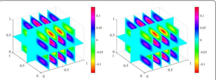
Figure 1The CFDS6-SSM solution (left-hand side) and error of CFDS6-SSM (right-hand side) whenJ= 41 and
t= 1 forSP1
Figure 2The E-CFDS6-SSM solution (left-hand side) and error of E-CFDS6-SSM (right-hand side) whenJ= 41 andt= 1 forSP1
and2. It also can be clearly seen that the E-SSM is almost as accurate as CFDS6-SSM and the computational times of E-CFDS6-CFDS6-SSM are less than those of CFDS6-CFDS6-SSM under the same number of nodes. In Fig.3, the error between CFDS6-SSM and E-CFDS6-SSM is no more than 3×10⁻⁷. It also can be found that the accuracy of E-CFDS6-SSM is almost identical to that of CFDS6-SSM. Besides, we also found that the order of con-vergence obtained by E-CFDS6-SSM and CFDS6-SSM is almost the same in Table2. In addition, it should be noted that our algorithm is easier to execute than the classical ADI algorithm.
Example2 Consider the following 2D parabolic equation (SP2):
⎧ ⎪ ⎪ ⎨ ⎪ ⎪ ⎩
(1 + 1 22)∂∂ut =∂
2u
∂x2 +∂ 2u
∂y2, (x,y)∈Ω, 0 <t≤2, u(x,y, 0) =sinxsin2y, (x,y)∈Ω,
u(x,y,t) = 0, (x,y)∈∂Ω, 0 <t≤2,
where Ω={(x,y); 0≤x≤2π, 0≤y≤2π},∂Ω denotes the boundary ofΩ. The exact solution isu(x,y,t) =e–tsinxsiny
2.
Table 1 The error of two different schemes forSP1att= 1
(xi,yi) CFDS6-SSM E-CFDS6-SSM DADI (error)
(0.4, 0.4) 1.0284e–06 1.2736e–06 1.5021e–02 (0.8, 0.8) 3.9282e–07 4.7769e–07 5.8051e–03 (1.2, 1.2) 3.9282e–07 4.7769e–07 5.5856e–03 (1.6, 1.6) 1.0284e–06 1.2736e–06 1.4801e–02
Nodes 41×41 41×41 201×201
Table 2 The convergence order and computational time forSP1att= 1
Nodes 11×11 21×21 41×41
CFDS6-SSM Max (error) 0.0441 2.1770e–04 1.3977e–06 Time (s) 10.099649 126.587866 416.107510
Order – 7.662 7.283
E-CFDS6-SSM Max (error) 0.0197 5.9319e–05 1.1370e–06 Time (s) 1.091099 51.221890 234.497833
Order – 8.375 5.705
Figure 3The error between the solution of CFDS6-SSM and solution of E-CFDS6-SSM whenJ= 41 andt= 1 for
SP1
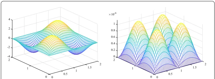
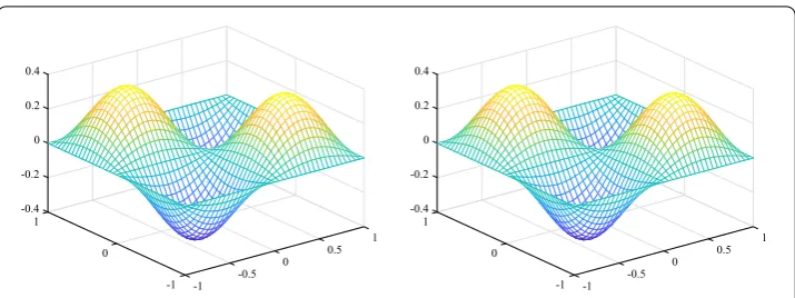
Figure 4The CFDS6-SSM solution (left-hand side) and error of CFDS6-SSM (right-hand side) whenJ= 41 and
t= 2 forSP2
Figure 5The E-CFDS6-SSM solution (left-hand side) and error of E-CFDS6-SSM (right-hand side) whenJ= 41 andt= 2 forSP2
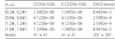
Table 3 The error of two different schemes forSP2att= 2
(xi,yi) CFDS6-SSM E-CFDS6-SSM DADI (error)
(0.2π, 0.2π) 1.3405e–06 1.3405e–06 8.4424e–5 (0.8π, 0.8π) 4.1228e–06 4.1230e–06 2.5983e–4 (1.2π, 1.2π) 4.1228e–06 4.1230e–06 2.5982e–4 (1.8π, 1.8π) 1.3396e–06 1.3405e–06 8.4416e–5
Nodes 41×41 41×41 201×201
Table 4 The convergence order and computational time forSP2att= 2
Nodes 21×21 41×41 81×81
CFDS6-SSM Max (error) 1.7206e–04 1.3604e–06 2.5087e–08 Time (s) 24.018882 52.936624 121.629286
Order – 6.982 5.761
E-CFDS6-SSM Max (error) 1.7280e–04 1.3614e–06 2.5088e–08
Time (s) 5.014861 12.554003 32.825120
Order – 6.988 5.762
our algorithm significantly improves the accuracy. In Fig.6, the error between CFDS6-SSM and E-CFDS6-CFDS6-SSM is no more than 1.5×10⁻⁹. It also indicated that the accuracy of E-CFDS6-SSM is almost identical to that of CFDS6-SSM under the same nodes and time step. Besides, we also give the order of convergence obtained by E-CFDS6-SSM and CFDS6-SSM in Table4, by which it can be seen clearly that the numerical results confirm the convergence with the rateO(h6) for this equation.
Example3 Consider the following 2D parabolic equation (SP3):
⎧ ⎪ ⎪ ⎨ ⎪ ⎪ ⎩
∂u
∂t – (
∂2u
∂x2 +∂ 2u
∂y2) =e–tsinxsiny, 0 <t≤2, u(x,y, 0) =sinxsiny, (x,y)∈Ω,
u(x,y,t) = 0, (x,y)∈∂Ω, 0 <t≤2,
whereΩ={(x,y); 0≤x≤π, 0≤y≤π},∂Ωdenotes the boundary ofΩ. The exact solu-tion isu(x,y,t) =e–tsinxsiny.
Figure 6The error between the solution of CFDS6-SSM and solution of E-CFDS6-SSM whenJ= 41 andt= 2 for
SP2
Figure 7The figure of CFDS6-SSM solution (left-hand side) and error of CFDS6-SSM (right-hand side) when
J= 41 andt= 2 forSP3
Figure 8The E-CFDS6-SSM solution (left-hand side) and error of E-CFDS6-SSM (right-hand side) whenJ= 41 andt= 2 forSP3
E-CFDS6-SSM and DADI with hx=hy= 0.005π andτ = 0.01, which indicates that our
Table 5 The error of two different schemes forSP3att= 2
(xi,yi) CFDS6-SSM E-CFDS6-SSM DADI (error)
(0.2π, 0.2π) 8.6691e–09 8.6716e–09 9.0752e–04 (0.4π, 0.4π) 2.2696e–08 2.2699e–08 2.3615e–03 (0.6π, 0.6π) 2.2696e–08 2.2699e–08 2.3437e–03 (0.8π, 0.8π) 8.6691e–09 8.6716e–09 8.8970e–04
Nodes 41×41 41×41 201×201
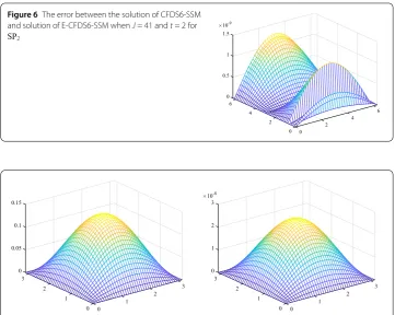
Table 6 The convergence order and computational time forSP3att= 2
Nodes 11×11 21×21 41×41
CFDS6-SSM Max (error) 1.7091e–04 1.3605e–06 2.5092e–08
Time (s) 1.008504 24.672396 56.174196
Order – 6.972 5.761
E-CFDS6-SSM Max (error) 1.7344e–04 1.3630e–06 2.5095e–08
Time (s) 0.525925 11.531699 31.044471
Order – 6.991 5.763
Figure 9The error between the solution of CFDS6-SSM and solution of E-CFDS6-SSM whenJ= 41 andt= 2 for
SP3
Example4 Consider the following 3D parabolic equation (SP4):
⎧ ⎪ ⎪ ⎨ ⎪ ⎪ ⎩
(1 +212 + 22)∂∂ut =∂ 2u
∂x2 +∂ 2u
∂y2 +∂ 2u
∂z2, (x,y,z)∈Ω, 0 <t≤2, u(x,y,z, 0) =sinxsiny2sin2z, (x,y,z)∈Ω,
u(x,y,z,t) = 0, (x,y,z)∈∂Ω, 0 <t≤2,
whereΩ={(x,y,z); 0≤x≤2π, 0≤y≤2π, 0≤z≤2π},∂Ωdenotes the boundary ofΩ. The exact solution isu(x,y,t) =e–tsinxsinysinz.
ob-Figure 10 The numerical solution of CFDS6-SSM (left-hand side) and E-CFDS6-SSM (right-hand side) when
J= 41 andt= 2 forSP4
Figure 11 The numerical solution of CFDS6-SSM (left-hand side) and E-CFDS6-SSM (right-hand side) when
J= 41,z= 0.4πandt= 2 forSP4
Table 7 The convergence order and computational time forSP4att= 2
Nodes 21×21×21 41×41×41 81×81×81
CFDS6-SSM Max (error) 2.7607e–04 4.5042e–06 7.1814e–08
Time (s) 10.010231 40.045140 89.493375
Order – 5.937 5.971
E-CFDS6-SSM Max (error) 7.7141e–04 4.2592e–06 7.1633e–08
Time (s) 5.005856 10.031937 22.965542
Order – 7.501 5.894
tained by E-CFDS6-SSM and CFDS6-SSM, which shows that the E-CFDS6-SSM still can produce very accurate solution.
Example5 Consider the following 3D parabolic equation (SP5):
⎧ ⎪ ⎪ ⎨ ⎪ ⎪ ⎩
∂u
∂t – (
∂2u
∂x2 +∂ 2u
∂y2 +∂ 2u
∂z2) =e–t(3π2– 1)sinπxsinπysinπz, (x,y,z)∈Ω, 0 <t≤1, u(x,y,z, 0) =sinπxsinπysinπz, (x,y,z)∈Ω,
u(x,y,z,t) = 0, (x,y,z)∈∂Ω, 0 <t≤1,
Figure 12 The error of CFDS6-SSM (left-hand side) and E-CFDS6-SSM (right-hand side) whenJ= 41,z= 0.4π andt= 2 forSP4
Figure 13 The error between the solution of CFDS6-SSM and solution of E-CFDS6-SSM whenJ= 41,z= 0.4πandt
= 2 forSP4
Figure 14 The numerical solution of CFDS6-SSM (left-hand side) and E-CFDS6-SSM (right-hand side) when
J= 41 andt= 1 forSP5
Figure 15 The numerical solution of CFDS6-SSM (left-hand side) and E-CFDS6-SSM (right-hand side) when
J= 41,z= –0.4 andt= 1 forSP5
Table 8 The convergence order and computational time forSP5att= 2
Nodes 11×11×11 21×21×21 41×41×41
CFDS6-SSM Max (error) 0.0021 6.3364e–06 1.1076e–07
Time (s) 5.139907 121.805555 351.633034
Order – 8.372 5.838
E-CFDS6-SSM Max (error) 3.6402e–04 4.0606e–06 1.1199e–07
Time (s) 1.008504 24.672396 56.174196
Order – 6.486 5.761
Figure 16 The error of CFDS6-SSM (left-hand side) and E-CFDS6-SSM (right-hand side) whenJ= 41,z= –0.4 andt= 1 forSP5
error between E-CFDS6-SSM and CFDS6-SSM is given. Besides, in Table8, we also gave the computational time and order of convergence obtained by E-SSM and CFDS6-SSM, which indicates that the E-CFDS6-SSM is more efficient than the CFDS6-SSM for solving the parabolic equation and E-CFDS6-SSM holds same accuracy.
Example6 Consider the following 3D parabolic equation (SP6):
⎧ ⎪ ⎪ ⎨ ⎪ ⎪ ⎩
∂u
∂t – (
∂2u
∂x2 +
∂2u
∂y2 +
∂2u
∂z2) = 2e–tsinxsinysinz, (x,y,z)∈Ω, 0 <t≤1, u(x,y,z, 0) =sinxsinysinz, (x,y,z)∈Ω,
Figure 17 The error between the solution of CFDS6-SSM and solution of E-CFDS6-SSM whenJ= 41,z= –0.4 andt
= 1 forSP5
Figure 18 The numerical solution of CFDS6-SSM (left-hand side) and E-CFDS6-SSM (right-hand side) when
J= 41 andt= 1 forSP6
Figure 19 The numerical solution of CFDS6-SSM (left-hand side) and E-CFDS6-SSM (right-hand side) when
J= 41,z= 0.4πandt= 1 forSP6
whereΩ={(x,y,z); 0≤x≤2π, 0≤y≤2π, 0≤z≤2π},∂Ωdenotes the boundary ofΩ. The exact solution isu(x,y,t) =e–tsinxsinysinz.
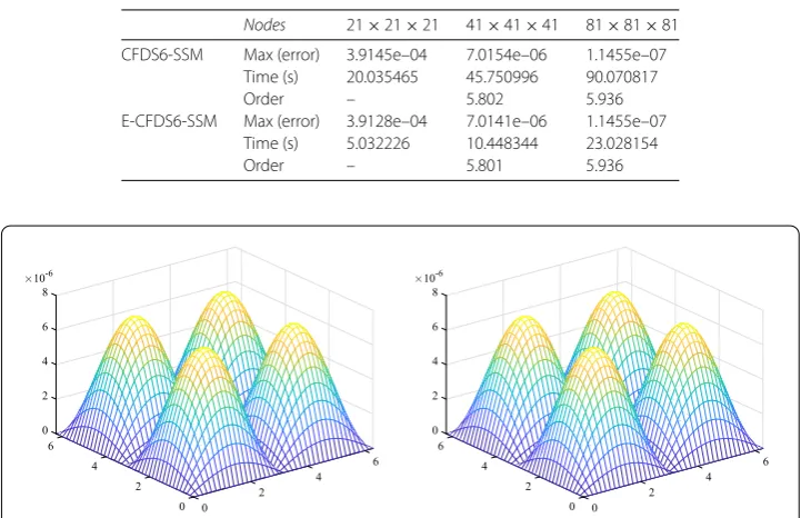
er-Table 9 The convergence order and computational time forSP6att= 1
Nodes 21×21×21 41×41×41 81×81×81
CFDS6-SSM Max (error) 3.9145e–04 7.0154e–06 1.1455e–07
Time (s) 20.035465 45.750996 90.070817
Order – 5.802 5.936
E-CFDS6-SSM Max (error) 3.9128e–04 7.0141e–06 1.1455e–07
Time (s) 5.032226 10.448344 23.028154
Order – 5.801 5.936
Figure 20 The error of CFDS6-SSM (left-hand side) and E-CFDS6-SSM (right-hand side) whenJ= 41,z= 0.4π andt= 1 forSP6
Figure 21 The error between the solution of CFDS6-SSM and solution of E-CFDS6-SSM whenJ= 41,z= 0.4πandt
= 1 forSP6
ror and point-wise absolute errors of CFDS6-SSM and E-CFDS6-SSM in Figs.20and21. It can be seen that the E-CFDS6-SSM is similar to CFDS6-SSM. Besides, in Table9, we also give the order of convergence obtained by E-CFDS6-SSM and CFDS6-SSM, which in-dicates that the E-CFDS6-SSM is not only more efficient than the CFDS6-SSM for solving the parabolic equation, but it holds the same accuracy.
5 Conclusions
E-CFDS6-SSM is greatly less than CFDS6-SSM and the whole process of implementation of E-CFDS6-SSM is simpler than CFDS6-SSM. We test our algorithm by six numerical experiments, which implies that the E-CFDS6-SSM has high efficiency and is reliable for solving the MDPE.
Appendix: The detailed implementation of ADI for 2D parabolic equation For the 2D problem
⎧
Firstly, define the following central difference operators:
⎧
We can rewrite Eq. (23) by these difference operators
uk+1
Then we have the formula
In order to obtain a collection of one-dimensional problems that can be solved by the tri-diagonal matrix, we add r1r2
4 δ
the right-hand side of Eq. (25). Then Eq. (25) can be written as
Then Eq. (26) also can be rewritten as
By introducing the variable Vi,j, the well-known Peaceman–Rachford scheme can be
It should be noticed that the boundary condition should be given in the first scheme of Eq. (28).
⎧ ⎨ ⎩
V0,j=12(1 +r22δ2y)uk0,j+12(1 –
r2
2δ2y)uk0,+1j ,
Vm,j=12(1 +r22δ2y)ukm,j+12(1 –
r2
2δ 2
y)ukm+1,j.
(29)
We assume theuki,jis given. In the first scheme of Eq. (28), we first fixj(1≤j≤n– 1), then the system consisting ofm– 1 equations withm– 1 unknowns can be solved to get theV. Similarly, we first fixi(1≤i≤m– 1), then, by theV, the system consisting ofn– 1 equations withn– 1 unknowns can be solved to get theuki,+1j .
Acknowledgements
The authors express their sincere thanks to the anonymous reviews for their valuable suggestions and corrections for improving the quality of this paper.
Funding
This work is financially supported by the Academic Mainstay Foundation of Hubei Province of China (No. D20171202), and the National Natural Science Foundation of China (Grant No. 11826208).
Availability of data and materials
Not applicable.
Competing interests
The authors declare that they have no competing interests.
Authors’ contributions
All authors contributed equally and significantly in writing this article. All authors read and approved the final manuscript.
Publisher’s Note
Springer Nature remains neutral with regard to jurisdictional claims in published maps and institutional affiliations.
Received: 15 February 2019 Accepted: 30 July 2019 References
1. Hammad, D.A., El-Azab, M.S.: 2N order compact finite difference scheme with collocation method for solving the generalized Burgers–Huxley and Burgers–Fisher equations. Appl. Math. Comput.258, 296–311 (2015)
2. Wang, H., Zhang, Y., Ma, X., Qiu, J., Liang, Y.: An efficient implementation of fourth-order compact finite difference scheme for Poisson equation with Dirichlet boundary conditions. Comput. Math. Appl.71, 1843–1860 (2016) 3. Mohebbi, A., Abbaszadeh, M., Dehghan, M.: Compact finite difference scheme and RBF meshless approach for
solving 2D Rayleigh–Stokes problem for a heated generalized second grade fluid with fractional derivatives. Comput. Methods Appl. Mech. Eng.264, 163–177 (2013)
4. Düring, B., Fournié, M., Heuer, C.: High-order compact finite difference schemes for option pricing in stochastic volatility models on non-uniform grids. J. Comput. Appl. Math.271, 247–266 (2014)
5. Chen, J., Ge, Y.: High order locally one-dimensional methods for solving two-dimensional parabolic equations. Adv. Differ. Equ.2018, 361 (2018)
6. Bhatt, H.P., Khaliq, A.Q.M.: Fourth-order compact schemes for the numerical simulation of coupled Burgers’ equation. Comput. Phys. Commun.200, 117–138 (2016)
7. Sari, M., Gürarslan, G.: A sixth-order compact finite difference scheme to the numerical solutions of Burgers’ equation. Appl. Math. Comput.208, 475–483 (2009)
8. Zhang, X., Zhang, P.: A reduced high-order compact finite difference scheme based on proper orthogonal decomposition technique for KdV equation. Appl. Math. Comput.339, 535–545 (2018)
9. Liang, Y.C., Lee, H.P., Lim, S.P., Lin, W.Z., Lee, K.H., Wu, C.G.: Proper orthogonal decomposition and its applications—Part I: theory. J. Sound Vib.252, 527–544 (2002)
10. Rathinam, M., Petzold, L.R.: A new look at proper orthogonal decomposition. SIAM J. Numer. Anal.41, 1893–1925 (2003)
11. Kerschen, G., Golinval, J.-C., Vakakis, A.F., Bergman, L.A.: The method of proper orthogonal decomposition for dynamical characterization and order reduction of mechanical systems: an overview. Nonlinear Dyn.41, 147–169 (2005)
12. Ullmann, S., Rotkvic, M., Lang, J.: POD-Galerkin reduced-order modeling with adaptive finite element snapshots. J. Comput. Phys.325, 244–258 (2016)
14. An, J., Luo, Z., Li, H., Sun, P.: Reduced-order extrapolation spectral-finite difference scheme based on POD method and error estimation for three-dimensional parabolic equation. Front. Math. China10, 1025–1040 (2015)
15. Luo, Z., Li, H., Sun, P.: A reduced-order Crank–Nicolson finite volume element formulation based on POD method for parabolic equations. Appl. Math. Comput.219, 5887–5900 (2013)
16. Peaceman, D.W., Rachford, H.H. Jr.: The numerical solution of parabolic and elliptic differential equations. J. Soc. Ind. Appl. Math.3, 28–41 (1955)
17. Seydao ˘glu, M.: An accurate approximation algorithm for Burgers’ equation in the presence of small viscosity. J. Comput. Appl. Math.344, 473–481 (2018)
18. Gidey, H.H., Reddy, B.D.: Operator-splitting methods for the 2D convective Cahn–Hilliard equation. Comput. Math. Appl.77, 3128–3153 (2019)
19. Sun, J., Eichholz, J.A.: Splitting methods for differential approximations of the radiative transfer equation. Appl. Math. Comput.322, 140–150 (2018)
20. Einkemmer, L., Moccaldi, M., Ostermann, A.: Efficient boundary corrected Strang splitting. Appl. Math. Comput.332, 76–89 (2018)
21. Li, J., Chen, Y., Liu, G.: High-order compact ADI methods for parabolic equations. Comput. Math. Appl.52, 1343–1356 (2006)
22. Li, J., Visbal, M.R.: High-order compact schemes for nonlinear dispersive waves. J. Sci. Comput.26, 1–23 (2006) 23. Li, J.: High-order finite difference schemes for differential equations containing higher derivatives. Appl. Math.
Comput.171, 1157–1176 (2005)
24. Sun, P., Luo, Z., Zhou, Y.: Some reduced finite difference schemes based on a proper orthogonal decomposition technique for parabolic equations. Appl. Numer. Math.60, 154–164 (2010)
25. Luo, Z., Yang, X., Zhou, Y.: A reduced finite difference scheme based on singular value decomposition and proper orthogonal decomposition for Burgers equation. J. Comput. Appl. Math.229, 97–107 (2009)