Detection of jamming attacks in 802 11b wireless networks

(1)

R E S E A R C H

Open Access

Detection of jamming attacks in 802.11b

wireless networks

Nadeem Sufyan

1*

, Nazar Abbass Saqib

2

and Muhammad Zia

3

Abstract

The work in this paper is about to detect and classify jamming attacks in 802.11b wireless networks. The number of jamming detection and classification techniques has been proposed in the literature. Majority of them model individual parameters like signal strength, carrier sensing time, and packet delivery ratio to detect the presence of a jammer and to classify the jamming attacks. The demonstrated results by the authors are often overlapping as most of the jamming regions are closely marked, and they do not help to clearly distinguish different jamming mechanisms. We investigate a multi-modal scheme that models different jamming attacks by discovering the correlation between three parameters: packet delivery ratio, signal strength variation, and pulse width of the received signal. Based on that, profiles are generated in normal scenarios during training sessions which are then compared with test sessions to detect and classify jamming attacks. Our proposed model helps in clearly differentiating the jammed regions for various types of jamming attacks. In addition, it is equally effective for both the protocol-aware and protocol-unaware jammers. The reported results are not based on simulations, but a test-bed was established to experiment real scenarios demonstrating significant enhancements in previous results reported in the literature.

Keywords: Jamming attacks; Detection and classification; 802.11 wireless networks

1 Introduction

Wireless networks make use of shared transmission medium; therefore, they are open to several malicious attacks. An attacker with a radio transceiver intercepts a transmission, injects spurious packets, and blocks or jams the legitimate transmission. Jammers disrupt the wireless communication by generating high-power noise across the entire bandwidth near the transmitting and receiv-ing nodes. Since jammreceiv-ing attacks drastically degrade the performance of wireless networks, some effective mecha-nisms are required to detect their presence and to avoid them. Constant, deceptive, reactive, intelligent, and ran-dom jammers are few jamming techniques used in wire-less medium. All of them can partially or fully jam the link at varying level of detection probabilities.

Accurate detection of radio jamming attacks is chal-lenging in mission critical scenarios. Many detection techniques have been proposed in the literature, but the

*Correspondence: [email protected]

1School of Electrical Engineering and Computer Science (SEECS), National University of Science and Technology (NUST), Sector H-12, Islamabad 44000, Pakistan

Full list of author information is available at the end of the article

precision component is always an issue. Some of them either produce high false alarm rates or do partial detec-tion of jamming attacks. Moreover, the results are based on simulations [1-7]. After detection, classification of jam-ming attacks is necessary to launch appropriate recovery techniques like channel hopping or spatial retreat. The classification of jamming attacks plays an important role not only to differentiate them from each other but also to identify different network performance degradation phenomena like network congestion or channel fading.

1.1 Our contribution

As earlier said, the reported work in the literature mainly focus on the classification of jamming attacks based on packet delivery ratio (PDR), signal strength (SS), or carrier sensing time (CST) individually. Accu-rate detection of jamming attacks based on single detec-tion parameter is not too accurate [1]. Various models based on two parameters have been proposed [1,3-5]. The detection of jamming based on PDR in consis-tence with signal strength and location is discussed in [1]. Authors in [1] identified jammed and non-jammed regions, but they did not distinguish different types

(2)

of jamming attacks. In [3], a drop in PDR is checked by considering the correlation coefficient between error and correct reception time, but that works for reactive jammers only. Another technique for detection based on fabricated clear-to-send (CTS) packets is discussed in [4]; however, it is more promising to intelligent jamming.

Authors in [5] observe the deferred transmissions. When PDR drops, the average number of transmission attempts per successful transmission is checked. Then, the decision of jamming or no jamming is taken based on the predefined threshold values. The PDR in corre-sponding with signal-to-noise ratio (SNR) is checked in [6], and the presence of a jammer is declared based on predefined threshold values. Authors also use the net-work throughput for the given number of nodes with fixed transmission probability as a detection parameter. The approach works fine; however, it needs more explanation for the cases when the SNR is low and the network is congested.

The jamming detection techniques reported in the lit-erature are of specific types. Authors have mainly worked on a particular jamming attack, and therefore, the classifi-cation of different attacks remained relatively less studied. The development of multi-modal detection technique can help in detecting jamming attacks with lower false alarm rate and high precision. In our work, we propose a three-dimensional model based on signal strength, PDR, and pulse width (PW) of the signal resulting in a significant improvement in accuracy and also to classify jamming attacks in a better way.

1.2 Outline

The rest of this article is organized as follows. Section 2 provides relevant definitions, terms, and metrics to char-acterize the jamming attacks. Section 3 provides a brief summary of previous work done on jamming detection and classification. In Section 4, we explain our proposed model for both the detection and classification of jam-ming attacks. An analysis on the achieved results is pre-sented in Section 6. Finally, conclusions are drawn in Section 7.

2 Definitions and metrics to measure

This section provides definitions of related parameters and explains types of jamming attacks. It also provides metrics to characterize jamming attacks.

2.1 Definitions

2.1.1 Packet delivery ratio

It is the ratio of the total number of packets correctly received to the total number of packets received. For an environment with noise and interference, the PDR is mea-sured at the receiver side as the ratio of number of packets

received that pass cyclic redundancy check (CRC) to the total number of packets received.

2.1.2 Packet sent ratio

Packet sent ratio (PSR) is measured at the transmitter side. It is the total number of acknowledgments (ACKs) packets received to the total number of packets transmitted.

2.1.3 Carrier sensing time

It is the time a station has to wait for the channel to get idle to start its transmission.

2.1.4 Signal strength

It is the signal power that is observed on the receiver end. Signal strength can be used as a detection parameter [1]. There are two approaches that are used to characterize the variation in signal strength: (1) average value of signal strength in time window and (2) spectral discrimination technique.

2.2 Types of jamming attacks 2.2.1 Constant jammers

A constant jammer continuously produces high-power noise that represents random bits. The bit generator does not follow any media access control (MAC) protocol and operates independent of the channel sensing or traffic on the channel.

2.2.2 Random jammers

A random jammer operates randomly in both sleep and jam intervals. During sleep interval, it sleeps irrespective of any traffic on the network, and during jam interval, it acts as a constant or reactive jammer. That jammer does not follow any MAC protocol. The PDR increases when the sleep interval increases and the packet size decreases.

2.2.3 Deceptive jammers

These jammers continuously send illegitimate packets so that the channel appears busy to the legitimate nodes. They are protocol aware and increase carrier sensing time for the legitimate nodes indefinitely. The difference between a deceptive and a constant jammer is that a con-stant jammer sends random bits continuously while a deceptive jammer sends packets which appear legitimate to the receiver.

2.2.4 Reactive jammers

(3)

2.2.5 Shot noise-based intelligent jammers

Shot noise-based intelligent jammers are protocol-aware jammers that just beat forward error correction (FEC) scheme used at physical and MAC layers [8]. IEEE 802.11b networks use convolutional coding at the physical layer. Single continuous pulse interfering legitimate packet can completely drop it if it is able to beat the FEC scheme used in the packet [7,9].

2.3 Characterizing jamming attacks

A jamming attack can be detected easily, less effective, energy efficient, or protocol aware. How to characterize a jamming attack? There are a few commonly used metrics characterizing the jamming attacks:

• Least detection probability

• Stealthy against detectors

• Completely denial of service like constant jammers

• Protocol aware so that they are less likely to detect

• Authentication of users

• Strength against FEC codes

• Strength at physical layer to beat channel coding techniques

• Energy conservation is to get highest jamming efficiency with least energy used

The type of metrics also depends on the application in consideration. Energy efficiency is an important metric for all the jammers specifically in jamming the sensor net-works for a long time. Strong denial of service is critical in war situations. Least probability of detection is desired for jammers if they have to keep for a long time in opponent areas safely. FEC schemes increase resilience of packet against errors. Strong FEC codes can be compromised with constant or intelligent jamming.

Similarly, metrics to efficient and accurate detection of jamming attacks are as follows:

• Low false alarm rate

• Proactive detection

• Least computational cost

• Quick detection

3 Literature review

PDR, PSR, CST, and SS are important measures to detect jamming attacks. These parameters are influenced by channel fading, network congestion, or link failure. Afore-mentioned jamming detection techniques have been dis-cussed in [1]. Adaptive threshold like in BMAC protocol is suggested in [1], but it has the drawback of continu-ously increasing the transmission power, eventually jam-mer blasting at channel and detector which shows the channel idle. Two signal strength measurements are taken into consideration. The basic average for energy detec-tion fails for a constant jammer. The technique of spectral

discrimination is used which shows that if higher order crossing is used, then it works for constant and deceptive jammers but cannot distinguish random and reactive jam-mers. CST is taken as another measure that is the time a node has to wait for the channel to start its transmission. It is observed that under network congestion, the CST is greater than those of random and reactive jammers.

Another detection strategy using PDR with two consis-tency checks, i.e., signal strength consisconsis-tency check and location consistency check (LCC), is proposed in [1]. If signal strength is higher, then PDR must be high while converse is not true. In case of LCC, an assumption is taken that all nodes in the network have their neighbor-hood information from their upper routing layer. If a node observes low PDR, it compares it with that of its neighbor and decides whether the channel is jammed or not. More-over, the neighboring nodes have to pass the location and update messages periodically about their new location. This is communication overhead. The effectiveness of methods in [1] is based on the analysis of the large amount of data collected in all possible scenarios. Thus, they are not designed as real-time methods. Another disadvan-tage is that the jamming detection method and counter-measure are separately considered so that the problems are simplified, but the network performances are not optimized.

(4)

inspection scheme that uses two-hop neighborhood infor-mation. The main idea is to compare the destination field on the CTS frame with the neighborhood informa-tion. The targeted node sends a clear reservation (CR) message back to all neighbors, and all nodes reset their values to previous NAV values. However, it uses two-hop neighborhood information that all nodes must maintain using periodic ‘HELLO’ messages so that the freshness of information could be maintained. Also, the node get-ting the fabricated CTS message with its ID as targeget-ting address sends back a CR message. Hence, there is a com-munication overhead in this technique. This technique also suffers from partial detection of a jamming attack, a portion of the network remains jammed, and other recovers from a jamming attack and works perfectly. Cell breathing is a new detection and recovery technique dis-cussed in [5] not only for the case of jammers but also for normal network operations to increase the network throughput. This approach works for constant jammer detection only and not for protocol-aware jammers. It is based on the number of frames transmitted per total attempts of transmission. If the transmission attempts are above a predefined threshold, the node is consid-ered jammed. After jammer detection, cell breathing is used to increase or decrease the transmission power of the access point so that the jammer may be kept away from the range of the access point. This not only helps in mitigating the jamming attack but also load balance the network throughput. Since the technique used in [1] sug-gests collection of large amount of data before analysis, [6] proposed a model-based jamming detection technique for wireless networks. Without prior knowledge of the net-work status, a head station can detect a jamming attack based on PDR observed for a certain value of SNR. How-ever, it is hard to tell whether the drop in PDR is due to network congestion or high SNR value. It then sug-gested the network throughput as a measure of jamming detection. It shows that for the given values of SNR and probability of successful transmission, the rate of change of the network throughput first increases with the num-ber of nodes in the network and reaches a peak value and then drops almost like a straight line. It used expected and observed throughput with marginal threshold values to detect jamming. However, this marginal threshold varies with network environments. Once the attack is detected, it uses a self-healing approach based on runtime channel allocation algorithm to dynamically assign the most opti-mal second channel with a best switching probability that minimizes transient time to stable state. However, this will work only for wide-band jammers where the num-ber of channels with reasonable frequency separation is available. The idea of shot noise-based protocol-aware intelligent jamming that is presented in [9] is claimed to be the most energy efficient and with lesser probability

of detection. In this technique, the jammer captures the NAV value of packet and hence transmission length. Dur-ing the packet transmission, jammer sends a high-power pulse with enough width that corrupts enough bits so that FEC would be exhausted, checksum would not be passed at MAC layer and the packet drops ultimately. Since the sender would not get the ACK so it will retransmit the packet. In [10], the PDR is considered as the detection parameter and showed that PDR is 78% under normal net-work operation. However, effects of channel fading, poor link, and network congestion could be other causes of drop in PDR.

4 The proposed system model

Our proposed model of RF jamming detects the presence of the jammers and also to classify them. The model is based on multi-modal approach that incorporates PDR and signal strength as the detection parameters. The PDR is computed over the given sample window of time. Sig-nal strength variation (S) and PW are the model-specific parameters. Signal strength variation (S) is the change in signal strength taken in dB, i.e., (S) = SSobserved -SSnetwork, whereSSnetwork is the signal strength achieved during training session without jamming and SSobserved is the signal strength observed when the network is sus-pected to be under attack. PW is the measure of time for which (S) is greater than the threshold value, and it is taken in microseconds.

The jamming pulse acts as high-power Gaussian noise which can appear several times over the channel. To com-pute, N samples of channel’s received energy s (t) are collected. The collected samples thus form a bigger win-dow of sampless(k),s(k - 1),...,s (k- N + 1), taken at consecutive smaller sampling time windows.

The detection is done using Equation 1.

T(k)=( k

j=k−N+1(s(j)2)

N ) (1)

T(k) is the average jamming pulse observed for window

of N samples. To decide the presence of a jammer,T(k)

is compared with some thresholdγ. The thresholdγ is carefully computed to avoid false detection.

The following are the relevant parameters collected by the detector in a given sample window of time to detect the jamming attack and its type: (1) PDR, (2) NAV value

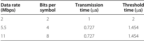
Table 1 IEEE 802.11b data rates and threshold time

Data rate Bits per Transmission Threshold

(Mbps) symbol time (μs) time (μs)

2 2 1 2

5.5 4 0.727 1.454

(5)

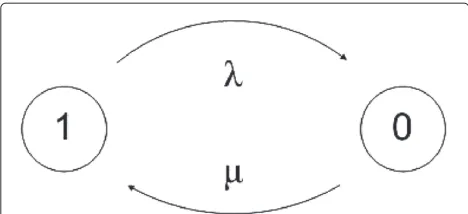
Figure 1State transition diagram for two-state random jammer.

of each packet transmission, (3)S, and (4) pulse width subject toS>0.

4.1 Computing data rate

Each packet on physical layer is composed of transmis-sion symbols. These transmistransmis-sion symbols are composed of bits. The transmission time of each symbol is depen-dent on data transmission rate. Hence, we first compute the data rate and subsequently the transmission time of each symbol. This computation is particularly of interest to intelligent jammers.

The data rate (DR) can be computed through the NAV value of each packet as shown in Table 1. The NAV value of each packet determines the transmission time of the packet which is there in the packet header. The data rate may be derived as follows:

DR=

The above derivations are valid for a MAC frame with the size of 2,312 bytes [9]. NAV value varies based on the packet size and the data transmission rate.

The PDR of the given sampling window can be com-puted as follows:

PDR=(1−Pj)(1−Pc), (3)

wherePjis the jamming probability computed for the dif-ferent jammers in the subsequent sections andPc is the collision probability of the packets when there are many transmitting nodes at the same time. Since, in our exper-iments, single transmitter and receiver are involved,Pcis always zero. However, it comes into consideration when the number of contending stations for the channel is more than one [11].

The jamming rate is the rate the jammer jams the chan-nel. Ifx is the time for whichS > 0 andyis the total sampling window time, then, it is written as follows:

Rj= x

y, (4)

where Rj is the jamming rate. For example, if jamming pulse lasts for 1μs in a total window of 1,000μs,Rjis said to be 1/1,000. For a constant jammer, because of continu-ous transmission of jamming pulse, the rate is 1. Jamming rateRjfor the timeTcan be derived through the following equation: the sub-window time during whichS>0.Tis the total sample window time.

4.2 Computing jamming probability

Jammers are classified into two major classes: channel aware and channel unaware. (1) Channel-aware jammers continuously sense the channel and send jamming pulses when the packet is transmitted. (2) Channel-unaware jam-mers do not sense the channel before sending the jamming pulse and independently jam the channel irrespective of the transmission or not on channel. To model the behavior of both types of jammers, we take assumptions that the (1) transmitter is operating in saturated mode and the chan-nel always have a packet on it. (2) For any PW of jammer, S> γ for the pulse duration, whereγ is the threshold defined in Equation 1.

Table 2 Summary of PDR,S, and pulse width

Number PW (μs) Sleep interval (μs) PDR Jammer type Data rate (Mbps)

1 1,000 1 0 Constant Any

(6)

0 10 20 30 40 50 60 70 80 90 100 0

100 200 300 400 500 600 700 800 900 1000

PDR (%)

Pulse Width (micro sec)

Constant Jammer

Experiment Normal

Normal Network Constant Jammer

Figure 2Detection of constant jamming attack.

4.2.1 Jamming probability of protocol-aware jammer

For protocol-aware jammers, the probabilityPof a packet to be jammed is conditioned on the fact that a packet is transmitting say denoted as transmission time of the packet (TPKT) and then the jamming pulse for the dura-tion of PW strikes the channel:

P(PW|TPKT)= P(PW∩TPKT)

P(TPKT) (6)

Each packet is composed of transmission symbols. The data bits in each symbol depend on the data rate. The

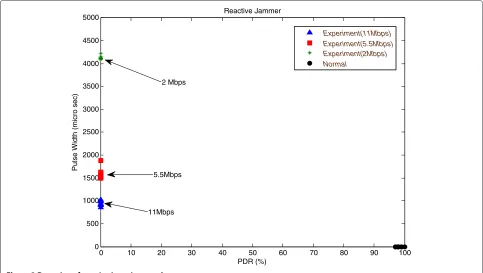
0 10 20 30 40 50 60 70 80 90 100

0 500 1000 1500 2000 2500 3000 3500 4000 4500 5000

PDR (%)

Reactive Jammer

Experiment(11Mbps) Experiment(5.5Mbps) Experiment(2Mbps) Normal

2 Mbps

5.5Mbps

11Mbps

(7)

0 10 20 30 40 50 60 70 80 90 100 0

1 2 3 4 5 6 7 8 9 10

PDR (%)

Shot Noise Based Intelligent jammer

Experiment(11Mbps) Experiment(5.5Mbps) Experiment(2Mbps) Normal

Figure 4Detection of shot noise jamming attack.

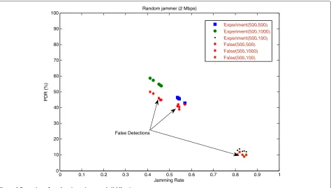
0 0.1 0.2 0.3 0.4 0.5 0.6 0.7 0.8 0.9 1 0

10 20 30 40 50 60 70 80 90 100

Jamming Rate

PDR (%)

Random jammer (2 Mbps)

Experiment(500,500) Experiment(500,1000) Experiment(500,100) False(500,500) False(500,1000) False(500,100)

False Detections

(8)

0 0.1 0.2 0.3 0.4 0.5 0.6 0.7 0.8 0.9 1 0

10 20 30 40 50 60 70 80 90 100

Jamming Rate

PDR (%)

Random jammer (5.5 Mbps)

False Detection

Figure 6Detection of random jamming attack (5.5 Mbps).

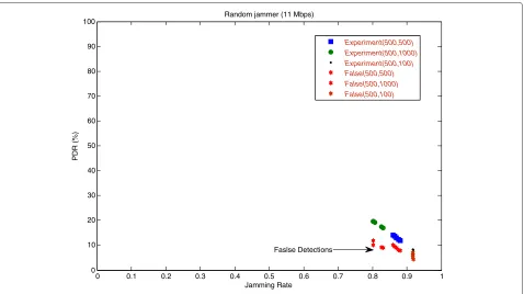
0 0.1 0.2 0.3 0.4 0.5 0.6 0.7 0.8 0.9 1 0

10 20 30 40 50 60 70 80 90 100

Jamming Rate

PDR (%)

Random jammer (11 Mbps)

Faslse Detections

(9)

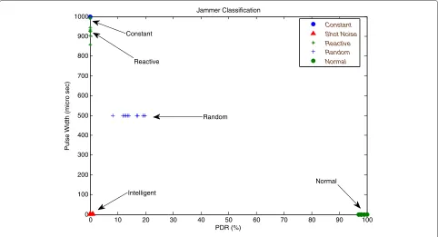
0 10 20 30 40 50 60 70 80 90 100 0

100 200 300 400 500 600 700 800 900 1000

PDR (%)

Jammer Classification

Constant Shot Noise Reactive Random Normal

Constant

Reactive

Random

Intelligent

Normal

Figure 8Detection and classification of four jamming attacks.

transmission time of each symbol,Tsymbol, is computed as follows:

Tsymbol= Nb

DR, (7)

whereNb is the number of data bits in each symbol and DR is data rate at which it is transmitted.

IEEE 802.11b does not use any FEC at the physical layer except channel codes (Barker and complementary code keying). It means that destroying one complete symbol will destroy the whole packet. Ideally, the threshold time (TH) for the jamming pulse required to destroy a packet is as follows:

TH=(2×Tsymbol)+GI (8)

where GI is the guard interval in two consecutive symbols. Guard interval is necessary to avoid intersymbol interfer-ence in two symbols. It is caused when symbols arrive at

the receiver from two different paths. Multiplication with 2 is to ensure that TH should be enough to completely overlap the symbol in air.

The duration of jamming pulse is different for different types of protocol-aware jammers. For the typical reactive jammer, the jammer PW is equal to the TPKT, i.e., jam-ming pulse lasts for the whole time of packet transmission. Whereas, for shot noise-based jammers, PW is greater than or equal to the TH as defined in Equation 9:

TPKT≥PW≥TH (9)

The difference in reactive and shot noise-based intelli-gent jammers is the PW. The shot noise-based jammers intelligently hit enough part of the transmission (data or ACK) such that the FEC scheme in the packet fails to recover the packet at the receiver side. Hence, with relatively lesser detection probability and higher energy efficiency, same jamming efficiency is achieved as that of the reactive jammer.

Table 3 IEEE 802.11b channel coding at physical layer

Data rate Code length Modulation Modulation rate Symbol rate (Msps) Bits per symbol

1 Mbps 11-Barker DBPSK 11,000,000 1 1

2 Mbps 11-Barker DQPSK 11,000,000 1 2

5.5 Mbps 8-CCK DQPSK 11,000,000 1.375 4

(10)

Table 4 Standard deviation between different jammers

Jammer Constant Random Reactive Intelligent

512.98 239.66 2118.71 2.52

Constant 512.98 316.67 2,072.98 212.32

Random 497.48 239.66 2,084 105.63

Reactive 92.17 1,134 2,113.61 879.41

Shot noise 509.27 240.61 2,104.52 2.49

The jamming probability of the protocol-aware jammers is subject to the condition of Equation 6, and it can be computed as follows:

whereK is the number of effected packets andN is the total number of packets in the sampling window.

4.2.2 Jamming probability of protocol-unaware jammers

The following are the jamming probability of protocol-unaware jammers:

• Constant jammer: the jamming probability of constant jammer is one. This is because the fact that it continuously transmits random bits during the whole observation window, and the channel appears always busy to legitimate nodes for transmission.

• Random jammer: random jammers jam the channel

independent of sleep and jam intervals of the transmission during a time window and behave exactly as constant jammer if sleep interval is zero during the time window. Consider a random jammer that acts as two-state continuous time Markov chain process as shown in Figure 1. It sleeps with

exponential amount of time with mean1_λ, whereλis

the sleeping rate and jams the exponential amount of time with mean_μ1, whereμis the jamming rate. The jammer jams and sleeps iteratively. Consider that the jammer is jamming initially att = 0, what is the steady state probability that the jammer will be jamming or sleeping at timet?

Where,

State 1: jam state, MTTJ (mean time to jam)=1/μ State 0: sleep state, MTTS (mean time to sleep)= 1/λ

For random jammer operating in the steady state, the global balance equations for both states are as follows:

λπ₁=μπ₀ (12)

μπ0=λπ1 (13)

whereπ0andπ1are the proportions of time the jammer spends in state {0,1}. Since both values in Equations 12 and 13 are unknown, from the normalization condition, we know that,

Equations 15 and 16 provide a steady state probability for sleep and jam state.

Transient availability of each state is the rate of buildup for each state. Considering state 1, rate of buildup = rate of flow in−rate of flow out:

π₁(t)=μπ₀(t)−λπ₁(t) (17)

π₁(t)=μ−(λ−μ)π1(t) (18)

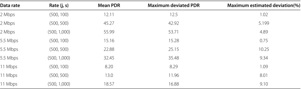
Table 5 Random jammer estimated PDR variation from mean

Data rate Rate (j, s) Mean PDR Maximum deviated PDR Maximum estimated deviation(%)

2 Mbps (500, 100) 12.11 12.5 1.02

2 Mbps (500, 500) 45.27 42.92 5.199

2 Mbps (500, 1,000) 55.99 53.71 4.89

5.5 Mbps (500, 100) 15.16 15.28 0.75

5.5 Mbps (500, 500) 22.88 25.15 10.25

5.5 Mbps (500, 1,000) 32.45 35.48 9.34

11 Mbps (500, 100) 8.20 8.29 1.09

11 Mbps (500, 500) 13.0 11.96 8.01

(11)

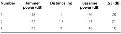
Table 6 No transmission, only jammer and detector

Number Jammer Distance (m) Baseline S(dB)

power (dB) power (dB)

1 -18 1 -46 28

2 -22 1.5 -43 21

3 -24 2 -39 15

Sinceπ₁(0) =1 and further solving Equation 18 yields the following [12]:

π1(t)= μ μ+λ+

λ μ+λexp

−(μ+λ)t ₍₁₉₎

and,

π0(t)= λ μ+λ+

μ μ+λexp

−(μ+λ)t ₍₂₀₎

Equations 19 and 20 give transient probability for jam and sleep state, respectively, at time t. However, for the system to be in steady state, for large value of t, Equation 19 is reduced to:

lim

t→∞π1(t)=

μ

μ+λ (21)

That is equivalent to Equation 15. Equations 15 and 16 give the probability of random jammer to remain in any of the two states.

4.3 Classification of jamming attacks

Identifying the type of jamming attacks is necessary to take appropriate recovery technique. For two stations in network, single transmitter and receiver, collision proba-bilityPc=0 and Equation 3 is reduced to:

PDR=(1−Pj) (22)

wherePjis the jamming probability computed for differ-ent jammers. The value ofPjfor constant jammer is always one; PDR is always observed to be zero. The jamming probability for intelligent and reactive jammers is com-puted in Equation 10. For the random jammer that jams and sleeps for exponential amount of time, Equation 15 computes the steady state jamming probability.

The types of jamming attacks are classified based on PDR and PW. Equation 23 acts as a classification equation based on Equation 22:

PDR

⎧ ⎪ ⎪ ⎪ ⎨ ⎪ ⎪ ⎪ ⎩

=0, PW=TH, ⇒Shot noise jammer =0, PW=TPKT, ⇒Reactive jammer =0, PW=Twin, ⇒Constant jammer ≥0, PW=X±σ, ⇒Random jammer

(23)

whereTwinis the time of whole sampling window,Xis the mean jamming pulse width observed for random jammer andσis the threshold value around it.

(12)

Figure 10Signal strength variation at 1.5 m.

(13)

Table 7 Legitimate transmission, jammer and detector

Number Jammer Distance (m) Baseline S(dB)

power (dB) power (dB)

1 -17 1 -35 18

2 -23 1.5 -33 10

3 -24 2 -32 8

It is important to note that the selection ofσ is a bit tricky, and it is dependent on the network. For example, in our experiments, we find that the drop in the PDR caused by the random jammer is 5.199% when the jammer is operating withTsandTjas [500,500]μs each at the DR of 2 Mbps. Therefore, we choseσ as 6%.

5 Experimental setup

We build a test bed for four jammers that are constant, random, reactive, and intelligent. The purpose of this pro-totype is to validate our analytical results with real-world experimental results. The test bed is based on Univer-sal Software Radio Peripheral (USRP) and GNU Radio for jammer and detector [13]. Four types of jammers are implemented on USRP. We observed the influence on PDR at detector under different jamming scenarios with different jamming parameters (PW,S).

5.1 Setup

Our experimental setup consists of four nodes: one as transmitter, one as receiver, one as jammer, and one as detector. The transmitter and receiver are connected via D-Link 2.4 GHz wireless router dl-514 (D-Link, London, England) with infrastructure mode. Both nodes are equipped with dwl-650 PCMCIA wireless cards (D-Link) that can operate on all four data rates of 802.11b. Both nodes have Fedora 12.86 (Raleigh, NC, USA) as the operating system with kernel 2.6. It automatically detects the wireless card driver. Installation and working of dwl-650 drivers can be seen at [14]. The traffic between two machines is generated using PING utility with zero inter-packet interval, and the size of each inter-packet is kept as 1,024 bytes.

Both the jammer and detector use Fedora 12.86 oper-ating system and implements GNURadio-3.2.4 and USRP. The USRP kit has RFX-2400 daughter boards of range 2,400 to 2,500 MHz and VERT-2450 vertical antenna (Ettus, Mountain View, CA, USA). The jamming models

have been written in Python, Beaverton, USA. The detec-tor machine has wireshark and a packet capture tool installed on it.

Experiments are performed with different placements of all the four nodes. However, due to space constraints, all the nodes are placed in a circle of 1.5-m radius by plac-ing the wireless router at the center of the circle and all other nodes at the circumference of the circle. The jam-ming node is preferred to be kept near the receiver to affect PDR.

Ideal channel conditions are achieved by scanning the channel one by one for some time and pick up the one that is least affected from interference. Jamming pulse has the power ranging from 15 to 19 dB enough higher than the normal transmission. It is sufficient to corrupt the ongoing transmission.

5.2 Algorithm

Algorithm 1 explains the detection sequence. The text for the conditional statements is kept italic, and the remain-ing algorithm is in regular text format. The PDR of a node is obtained using the method MeasurePDR(). It is then compared with the predefined threshold value threshPDR. If PDR is lower than the threshold value, then the current signal strength variation S is com-pared with signal strength variation S in the nor-mal network. Next is to check the PDR in consistence with S using CheckPDRnSSvariation totalPDR, S. If it is found true that the symbol transmission time is obtained through GetSymbolTransmissionTime(), the packet transmission time is obtained through GetPack-etTransmissionTime(packetLength) and the pulse width using GetObservedPulseWidth() methods. The obtained PW is then compared with its predefined values for con-stant, random, reactive, and protocol-aware intelligent jammers.

The pseudocode of Algorithm 1 suggests that there are n statements. So the time complexity of the proposed algorithm isO(n).

5.3 Training the detector

In this phase, we train the detector for different jamming scenarios. The transmitter sends the legitimate packets to the receiver. The jammer jams it depending on the jam-ming technique being employed at that time. The receiver, on the other end, captures the packets. That process is

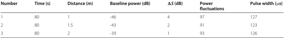
Table 8 No transmission, no jammer

Number Time (s) Distance (m) Baseline power (dB) S(dB) Power

fluctuations

Pulse width (μs)

1 80 1 -46 4 97 127

2 80 1.5 -43 2 91 123

(14)

Algorithm 1: Jammer detection and classification algorithm

Input: totalPDR(N) = MeasurePDR() : N∈Neighbors Output: Jammer Type Alert

if(totalPDR≤threshPDR)then S= SampleSignalStrength() -NormalSignalStrength()

PDRSSV = CheckPDRSSVariation(totalPDR,S) if(PDRSSV == false)then

Post NetworkError()

else if(PW == packetTT)then Post ReactiveJammed() end

else if(PW == ConstantJammed())then Post ConstantJamming()

end

else if(PW == RandomPulse())then sleepInterval = GetSleepInterval() if(sleepInterval > packetTT)then

totalPDR > 0else totalPDR == 0

repeated for 120 s for each jammer. During this time, the set of the entire packet influenced through jamming is created. Meanwhile, the detector measures the variation in signal strength (S) and also the PW. Based on the proposed multi-modal scheme, the area of occurrence of these parameters is determined for each type of jammer. Each detection area represents a type of jamming attack. This analogy helps in the detection of a jamming attack and classification.

The PDR of each session is measured using Wireshark that acts as a packet capturing tool to capture packets received at the network interface. The CRC of the packet is checked on reception, and the packets with bad CRC are listed and dropped. PDR is then measured as the num-ber of packets is correctly received to the total numnum-ber of packets received. The impact of signal strength vari-ation (S) is discussed in Section 5.3. PW is dependent

on the signal strength variation. Since the transmission power varies because of power fluctuations and external interference (Wi-Fi access point), signal strength varia-tion thresholdγ needs to be set.γ also depends on the distance between the jammer and the detector, transmis-sion power of the transmitter, and the amount of external interference.

Since pulse width is taken for signal strength vari-ation above a predefined threshold γ at defined dis-tance, the drop in PDR can be estimated. To validate the above argument, experiments are done for various jamming scenarios and the corresponding results are collected.

6 Analysis and results

We carried out multiple sessions for each type of jammer described in Section 2.2. As shown in Table 2, we mea-sure the (1) PW for different types of jammers, (2) impact on PDR, and (3) variation in signal strength (S) that is under normal and jammed scenarios by keeping the size of the packets as 1,024 bytes. For a given jammer type, each jamming session lasts for 120 s and the frequency is 2,450 MHz. The session is repeated for five times, and the average value is taken.

SIcis the sleep interval of channel, andσis the variation in pulse width observed.

6.1 Results

Figures 2, 3, 4, 5, 6, and 7 individually describes four jam-mers, and Figure 8 classifies four types of jammers and indicates the area where the type of jammer lies. In these figures, empirically gathered experimental results taken from test bed validate analytical counterparts. Figure 4 shows shot noise-based intelligent jammers where the TH is experienced lesser than that of our results. The reason for the increase in pulse width is channel coding robust-ness provided at different data rates. Another reason is the experienced throughput provided by commercial IEEE 802.11b wireless cards [15]. The actual throughput expe-rienced is around one-half of the one provided by the vendor. This is the reason of providing almost double jamming pulse to completely jam the packet.

Figure 5 indicates that high jamming efficiency can be achieved with very small jamming rate, i.e., almost zero PDR for different pulse widths.

It is to be noted that 802.11b does not have any FEC scheme at the physical layer [16]. However, it uses dif-ferent channel coding schemes for difdif-ferent data rates as shown in Table 3.

(15)

Figure 12Pulse width monitoring during training session.

with bad bytes pass to MAC layer. Since these packets cannot pass CRC check, hence these are discarded. It can also be inferred that the probability of packet drop increases/decreases with data rate, modulation [17], and coding techniques the transmission is using. It is also worth mentioning here that DSSS is relatively more robust than CCK because of 11 chips per bit that are spread on 22 MHz band. CCK uses 4 bits/8chips for 5.5 Mbps and 8 bits/8 chips for 11 Mbps. However, autocorrelation properties of CCK make it robust [18].

The standard deviation of ten experimental values of pulse width and PDR is given in the first row of Table 4. Subsequent rows provide variation in the standard devi-ation for the mean value of pulse width and PDR for the given jammer at a data rate of 2 Mbps.

Table 4 indicates the variation in the standard deviation. It is observed that the standard deviation of all four jam-mers differs significantly as indicated by the first row of Table 4. The impact on standard deviation for different jammers is shown in row 2 to row 5. It is computed if the mean value of pulse width and PDR for any other jam-mer under consideration is provided. It is observed that

the first two columns of the last row do not show signif-icant variation from the standard deviation value of con-stant and random jammers, respectively. Here, the pulse width of the different jammers is used as a classification parameter.

Reasonable estimates of PDR variation are required for random jammers. We developed a random jammer that operates in jam and sleep intervals iteratively. Jam and sleep rates follow exponential distribution and generate pseudorandom numbers around given jam and sleep rate. Table 5 indicates the maximum PDR variation from the mean value for the given (jam, sleep) rate at a specific data rate.

6.2 Assessment of false detections and signal strength variation

It is important to characterize the signal strength variation and false detections for accuracy assessment. The term baseline power is the power that the detector observes when no jamming activity on the channel is under obser-vation. This is the power observed when there is no transmission or transmission on the channel. Different

Table 9 Microwave oven and detector, no jammer

Number Distance (m) Frequency (MHz) External noise (dB) Baseline power (dB) S(dB)

1 1 2,450 -30 -46 16

2 1.5 2,450 -35 -46 11

(16)

Figure 13The spectral changes in the presence of high power external interference.

scenarios with multiple parameters are created to charac-terizeSand impact of distance.

6.2.1 No transmission, only jammer and detector

The experiment is done with single jammer and detector in the scenario. The distance in the jammer and detector varies from 1 to 2 m. The impact on signal strength is shown in Table 6.

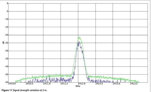
The impact on signal strength variation with distance can be seen from Figures 9, 10, and 11.

6.2.2 Legitimate transmission and jammer

The experiment is performed with one legitimate packet generator connected to the access point. The jammer and detector are placed at a distance changing from 1 to 2 m. The results are shown in Table 7.

It is important to observe in Table 7 that the baseline power alleviated from -35 to -32 dB for the distance of 1 to 2 m, respectively. The baseline power is actually the transmission power observed at the channel. Hence,S reduces from 18 to 8 dB as the distance increases from 1 to 2 m. This indicates careful selection of thresholdγ

to differentiate jamming from false detection for variable distance.

6.2.3 No transmission, no jammer

In this scenario, only the detector machine is active. It is created to observe the average number of power fluc-tuations and external interferences in a given window of time. The average pulse width time for fluctuations is also observed. The results are shown in Table 8.

Figure 12 shows the pulse width spectrum. It is taken at the detector machine during point-to-point transmission session.

Table 8 shows that PW, because unintentional exter-nal interference, is enough to drop an 802.11b packet at supported data rates. It is important that S is small. Many commercial wireless NICs have adaptive transmis-sion power and treat suchSas noise.

6.2.4 High-power external interference

It is important to characterize the intentional jamming attack from unintentional high-power noise interference. To produce external interference, a microwave oven

Table 10 Microwave oven, detector and jammer

Number Distance (m) Frequency (MHz) External noise (dB) Baseline power (dB) S(dB)

1 1 2450 -29 -46 17

2 1.5 2450 -26 -46 20

(17)

Table 11 False detection rate for random jammer

Data rate Rate (j, s) Mean PDR Observed PDR Noise active time (s) False detections (%)

2 Mbps (500, 100) 12.5 10 10 1.66

2 Mbps (500, 500) 45.27 41 10 4.5

2 Mbps (500, 1,000) 55 45 10 5.1

5.5 Mbps (500, 100) 15 11.28 10 1.83

5.5 Mbps (500, 500) 22.88 16 10 5.3

5.5 Mbps (500, 1,000) 32.45 21 10 5.92

11 Mbps (500, 100) 8.20 5.87 10 2.1

11 Mbps (500, 500) 12.63 8.1 10 5.43

11 Mbps (500, 1,000) 18.57 10.9 10 6.62

operating at 2,450 MHz is used. The oven is operated for 10 s during each monitoring session. Table 9 shows the spectrum change results when no jammer activates, and Figure 13 shows the spectral changes. Table 10 demonstrates the statistical results in the presence of a jammer.

Sin Table 9 is found to be close toSdue to a jammer in a given scenario. Since the external noise source acts as a constant jammer during activation time, it is difficult to classify the drop in PDR due to the constant jammer or external noise source. For random jammers, false detec-tions are shown from Figures 5, 6, and 7. The impact of high-power external noise on PDR of random jammer is shown in Table 11. It is evident that false detection rate increases with an increase in the high-power external noise operating at a distance for whichS≤γ.

7 Conclusion

The major contribution of the work is the classification of jamming attacks with accuracy and low false alarm rate. Instead of performing simulations, a real test bed is developed for launching different jamming attacks with software-defined radio on USRP. Similarly, the detector node equipped with USRP and Python scripts collected the readings. The experimental results are cross veri-fied with analytical results. This multi-modal detection scheme not only enhanced the accuracy of detection but also provided the classification of jamming attacks. It takes into account that PDR, signal strength variation, and pulse width yield results that comply with experimental results.

The proposed mathematical model is an attempt towards solid foundation for the classification of jamming attacks. Moreover, the experiments are done with single transmitter and receiver. It is extensible for more than two nodes to monitor the PDR and signal strength variation of transmitting nodes. Signal strength variation becomes complex when more than two transmitting nodes and a jammer are present on the channel. To study the change

of power levels in the presence of multiple stations and jammers, there could be another dimension for study. Another aspect is to mathematically model the collision probability and extend the equations that compute PDR. IEEE 802.11 g/n are not addressed in this paper. However, this work can be extended for these protocols.

Competing interests

The authors declare that they have no competing interests.

Author details

1_{School of Electrical Engineering and Computer Science (SEECS), National}

University of Science and Technology (NUST), Sector H-12, Islamabad 44000, Pakistan.2_{College of Electrical and Mechanical Engineering (CEME), National}

University of Science and Technology (NUST), Sector H-12, Islamabad 44000, Pakistan.3_{Department of Electronics, Quaid-i-Azam University, Islamabad}

45320, Pakistan.

Received: 12 February 2013 Accepted: 3 August 2013 Published: 15 August 2013

References

1. W Xu, W Trappe, Y Zhang, T Wood. The feasibility of launching and detecting jamming attacks in wireless networks, inProceedings of the 6th ACM International Symposium on Mobile ad hoc Networking and Computing (MobiHoc 2005) (New York,USA, May 2005), pp. 46–57

2. E Bayrataroglu, C King, X Liu, G Noubir, R Rajaraman, B Thapa. On the performance of IEEE 802.11 under jamming, inProceedings of the 27th Conference on Computer Communications(INFOCOM ’08) (Phoenix AZ, USA, 13–18 Apr 2008)

3. A Hamieh, J Ben-Othman. Detection of jamming attacks in wireless Ad Hoc networks using error distribution, inInternational Conference on Communications(ICC ’09) (Dresden, Germany, 14–18 Jun 2009), pp. 1–6 4. X Zou, J Deng. Detection of fabricated CTS packet attacks in wireless

LANs, inProceedings of the 7th_{International ICST Conference on} Heterogeneous Networking for Quality, Reliability, Security and Robustness (QSHINE ’10)(Houston,USA, 17–19 Nov 2010), pp. 105–115

5. X Zou, J Deng. Detecting and mitigating the impact of wideband jammers in IEEE 802.11 WLANS, inProceeding of the 6th_{International} Wireless Communications and Mobile Computing Conference(ACM New York, 2010), pp. 57–61

6. M Yu, W Su, M Zhou. A new approach to detect radio jamming attacks in wireless networks, inInternational Conference on Networking Sensing and Control(Chicago,USA, 10–12 Apr 2010), pp. 721–726

(18)

8. Wikipedia, Shot, ‘shot’, ‘Shot Noise’ . http://en.wikipedia.org/wiki/Shot. Accessed 23 Jun 2012

9. A Hussain, NA Saqib. Protocol aware shot-noise based radio frequency jamming method in 802.11 networks, inProceedings of the 8th

International Conference on Wireless and Optical Communications Networks (Paris,France, 24–26 May 2011), pp. 1–6

10. K Pelechrinis, M Iliofotou, V Krishnamurthy, Denial of service attacks in wireless networks: the case of jammers. Communications Surveys and Tutorials.13, 245–257 (2010)

11. G Bianchi, On performance analysis of the ieee802.11 distributed coordination function. IEEE J. Selected Areas, Commun.18(3) (2000) 12. SM Ross,Introduction to Probability Models, 9th edn. Chapter 6. (Academic

Press, Orlando, 2006), pp. 381-383

13. Ettus Research, USRP. https://www.ettus.com/product/details/UN210-KIT, Accessed 3 Mar 2012

14. PCMCIA, ‘waves’, ‘PCMCIA Drivers’. http://www.egr.msu.edu/waves/ people/Ali.htm, Accessed 9 Apr 2012

15. G Bianchi, A Di Stefano, C Giaconia, L Scalia, G Terrazzino, I Tinnirello. Experimental assessment of the backoff behavior of commercial IEEE 802.11b Network Cards, in26th IEEE International Conference on Computer Communications(Anchorage, Alaska, USA, 6–12 May 2007), pp. 1181–1189 16. O Alay, T Korakis, Y Wang, S Panwar. An experimental study of packet loss

and forward error correction in video multicast over IEEE 802.11b network, inProceedings of the 6th IEEE Consumer Communications and Networking Conference (CCNC 2009)(Las Vegas, Nevada, USA, 10–13 Jan 2009), pp. 1–5 17. Wikipedia, Modulation, ‘Modulation’. http://en.wikipedia.org/wiki/

Modulation. Accessed 23 Jun 2012

18. R Gummadi, D Wetherall, B Greenstein, S Seshan, Understanding and mitigating the impact of RF interference on 802.11 networks. SIGCOMM Comput. Commun. Rev.37, 385–396 (2007)

doi:10.1186/1687-1499-2013-208

Cite this article as:Sufyanet al.:Detection of jamming attacks in 802.11b wireless networks.EURASIP Journal on Wireless Communications and Network-ing20132013:208.