Interpolated PLSI for Learning Plausible Verb Arguments

Interpolated PLSI for Learning Plausible Verb Arguments

Hiram Calvoa, b, Kentaro Inuia, and Yuji Matsumotoa

a

Computational Linguistics, Nara Institute of Science and Technology, Takayama, Ikoma, Nara 630-0192, Japan

{calvo, inui, matsu}@is.naist.jp b

Artificial Intelligence, Center for Computing Research, National Polytechnic Institute, Mexico City, DF, 07738, Mexico

[email protected]

Abstract. Learning Plausible Verb Arguments allows to automatically learn what kind of activities, where and how, are performed by classes of entities from sparse argument co-occurrences with a verb; this information it is useful for sentence reconstruction tasks. Calvo et al. (2009b) propose a non language-dependent model based on the Word Space Model for calculating the plausibility of candidate arguments given one verb and one argument, and compare with the single latent variable PLSI algorithm method, outperforming it. In this work we replicate their experiments with a different corpus, and explore variants to the PLSI method in order to explore further capabilities of this latter widely used technique. Particularly, we propose using an interpolated PLSI scheme that allows the combination of multiple latent semantic variables, and validate it in a task of identifying the real dependency-pair triple with regard to an artificially created one, obtaining up to 83% recall.

Keywords: Plausible Verb Arguments, K-Nearest Neighbors algorithm, KNN, Distributional Thesaurus, Probabilistic Latent Semantic Indexing, PLSI.

1

Introduction

Plausible Verb Arguments information is helpful in sentence reconstruction tasks. For example: The boy plays with the ____ in the ____; A _____ eats grass; and I drank _____ in a glass. Several tasks have to deal with this common problem, for example, anaphora resolution would consist on finding the referenced objects: The boy plays with it there, It eats grass, I drank it in a glass. Information Retrieval applications look for answers to 5W questions such as ‘Who eats grass?’, “Where?”, “When?” (Parton et al., 2009). The answers to these questions are not always explicitly stated in a text, such as ‘Where do boys play usually using what?’, ‘What do boys usually play with?’, ‘What is usually drunk in a glass?’ therefore, additional common sense knowledge is needed to answer these questions. Our goal is to create a large database of this information so that plausibility can be tested for performing a variety of tasks. For other tasks that can use this kind of information, see Section 1.1.

This problem can be seen as collecting a large database of semantic frames with detailed categories and examples that fit these categories. For this purpose, recent works take advantage

∗ We thank the support of the Japanese Government and the Mexican Government (SNI, SIP-IPN, COFAA-IPN, and PIFI-IPN). Second author is a JSPS fellow. We also thank our anonymous reviewers for their useful comments and discussion.

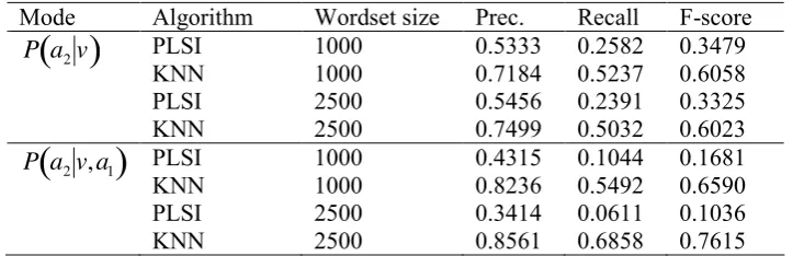
We want to know, given a verb and an argument

a

a

argument, i.e.

P a

(

v

,

a

)

relationships can be expressed as:

P v

(

,

a

,

a

)

=

P v

(

,

a

)

⋅

P a

(

v

,

a

)

, (1)

which can be estimated in several ways.

2.1

K-Nearest Neighbors Model

Uses the k nearest neighbors of each argument to find the plausibility of an unseen triple given its similarity to all triples present in the corpus, measuring this similarity between arguments. See Figure 1 for the pseudo-algorithm of this model.

for each triple <v,a1,a2> with observed count c,

for each argument a1,a2

Find its k most similar words a1s1…a1sk, a2s1…a2sk

with similarities s1s1, ..., s1sk and s2s1,...,s2sk.

Add votes for each new triple <v,a1si,a2sj> += c·s1si·s2sj

Figure 1: Pseudo-algorithm for the K-nearest neighbors DLM algorithm

As votes are accumulative, triples that have words with many similar words will get more votes.

Common similarity measures range from Euclidean distance, cosine and Jaccard’s coefficient (Lee, 1999), to measures such as Hindle’s measure and Lin’s measure (Lin, 1998a). Weeds and Weir (2003) show that the distributional measure with best performance is the Lin similarity, so this measure is used for smoothing the co-occurrence space, following the procedure as described by Lin (1998a).

2.2

PLSI – Probabilistic Latent Semantic Indexing

The probabilistic Latent Semantic Indexing Model (PLSI) was introduced in Hofmann (1999), arose from Latent Semantic Indexing (Deerwester et al., 1990). The model attempts to associate an unobserved class variable z∈Z={z1, ..., zk}, (in our case a generalization of correlation of the co-occurrence of v,a1 and a2), and two sets of observables: arguments, and verbs+arguments. In

terms of generative model it can be defined as follows: a v,a1 pair is selected with probability

P(v,a1), then a latent class z is selected with probability P(z|v,a1) and finally an argument a2 is

selected with probability P(a2|z). Calvo et al. (2009a) propose using PLSI (Hoffmann, 1999)

this said way, expressed also as (2).

P v

(

,

a

,

a

)

=

P z

( )

⋅

P a

(

z

)

⋅

Z

∑

P v

(

,

a

z

)

z is a latent variable capturing the correlation between a2 and the co-occurrence of (v,a1)

simultaneously. Using a single latent variable to correlate three variables may lead to a poor performance of PLSI, so that in next section we explore different ways of exploiting the smoothing by latent semantic variables.

2.3

iPLSI – interpolated PLSI

The previous PLSI formula originally used crushes the association of information from a2, and

v,a1 simultaneously into one single latent variable. This caused two problems: first, data

The following formula shows an interpolated way of estimating the probability of a triple based on the co-occurrences of its different pairs.

P

(

v

,

a

,

a

)

∝

f

(

v

,

a

)

f

(

a

)

+

f

(

v

,

a

)

f

(

a

)

+

f

(

a

,

a

)

f

(

a

)

fm

(

)

( )

(

)

∑

(

)

fn

(

)

( )

( )

∑

(

)

fo

(

)

( )

(

)

∑

(

)

(3)

where f(v), f(a₁), and f(a₂) are the observed probabilities of v, a₁ and a₂ respectively.

Additionally we test a model that considers additional information. See Eq. (4). Note that ai (the latent variable topics) should not be confused with a1 and a2 (the arguments).

P

(

v

,

a

,

a

)

≈

f

(

v

,

a

)

f

(

a

)

+

f

(

v

,

a

)

f

(

a

)

+

f

(

a

,

a

)

f

(

a

)

+

f

(

v

,

a

,

a

)

+

f

(

v

,

a

,

a

)

+

f

(

v

,

a

,

a

)

(

)

( )

(

)

a

∑

( )

fb

(

)

( )

(

)

∑

( )

fc

(

)

( )

(

)

∑

(

)

(4)

See the Figure 2 for a graphical representation of this concept. Each latent variable is represented by a letter in a small circle. Big circles surround the components of the dependency triple to be estimated. A black dot shows the co-occurrence of two variables. All of them contribute for the estimation of the triple v,a1,a2.

Figure 2: Graphical representation of iPLSI. The tuple v,a1,a2 is estimated by using latent variables based on pairs of two variables, and/or the pair of a variable and the co-ocurrence of two variables. See

3.2

Measuring the learning rate

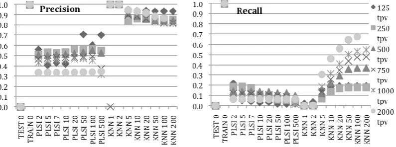
This experiment consisted on gradually increasing the number of triples from 125 to 2000 dependency triples per verb to examine the effects of using smaller corpora. Results are shown in Figure 3. In this figure KNN outperforms PLSI when adding more data. KNN precision is higher as well in all experiments. The best results for PLSI were obtained with 7 topics, while for KNN the best results were obtained using 200 neighbors.

Figure 3: Precision and Recall for the original PLSI and KNN with learning rate (each series has different number of triples per verb, tpv). The frequency threshold for triples was set to 4. The numbers

and the lower part show the number of topics for PLSI and the number of neighbors for KNN.

3.3

Results with no pre-filtering

Previous results used a pre-filtering threshold of 4, that is, triples with less than 4 occurrences

were discarded. Here we present results with no pre-filtering. In

Figure 4 results for KNN fall dramatically. PLSI is able to perform better with 20 topics. This suggests that PLSI is able to smooth better single occurrences of certain triples. KNN is better for working with frequently occurring triples. We require a method that can handle occurrences of un-frequent words, since pre-filtering implies a loss of data that could be useful afterwards. For example, consider that tezgüino is mentioned only once in the training test. We consider that it is important to be able to learn information for scarcely mentioned entities too. The next section presents results regarding to the improvement of using PLSI to handle non-filtered items.

Figure 4: Average of Precision and Recall for the original PLSI and KNN showing learning rate (each series has different number of triples per verb, tpv). No frequency threshold was used. The numbers and