Space and time efficient data structures in texture feature extraction

(1)

SPACE A N D TIM E E FFIC IE N T

DATA ST R U C T U R E S

IN

T E X T U R E FEA TU R E E X T R A C T IO N

Andrew E. Svolos

U n iversity College London

A T hesis S ub m itted to th e U niversity o f London for

th e D egree o f D octor of P h ilosop h y

(2)

ProQuest Number: U642772

INFORMATION TO ALL USERS

The quality of this reproduction is dependent upon the quality of the copy submitted.

In the unlikely event that the author did not send a complete manuscript and there are missing pages, these will be noted. Also, if material had to be removed,

a note will indicate the deletion.

uest.

ProQuest U642772

Published by ProQuest LLC(2015). Copyright of the Dissertation is held by the Author.

This work is protected against unauthorized copying under Title 17, United States Code. Microform Edition © ProQuest LLC.

ProQuest LLC

789 East Eisenhower Parkway P.O. Box 1346

(3)

A bstract

Texture feature extraction is a fundamental stage in texture image analysis. Therefore, the reduction of its computational time and storage requirements is an im portant objective.

The Spatial Grey Level Dependence Method (SGLDM) is one of the most im portant statistical texture analysis methods, especially in medical image pro cessing. Co-occurrence matrices are employed for its implementation. However, they are inefficient in terms of computational time and memory space require ments, due to their dependency on the number of grey levels in the entire image (grey level range). Since texture is usually measured in a small image region, a large amount of memory space is wasted while the computational time of the texture feature extraction operations is unnecessarily raised. Their inefficiency puts up barriers to the wider utilisation of the SGLDM in a real application environment, such as a clinical environment.

(4)

A cknow ledgem ents

I am indebted to my first supervisor, Prof. Andrew Todd-Pokropek, for his continuous support, guidance, and understanding. I am also very grateful to my second supervisor. Dr. Alfred Linney, for his support, encouragement, and especially his patience.

My special thanks to Dr. Jing Deng, Prof. Andrew Todd-Pokropek, Tryphon Lambrou, Chloe Hutton, and Dr. Joao C. Campos for providing me with the medical data and helping me with the region selection. The assistance from the prematurely deceased Dr. John Gardener in the ultrasonic analysis was extremely valuable. Especially, I would like to thank my colleague and friend, Tryphon Lambrou, for helping me with the classification experiments. Dr. Joanne M athias for her help and advice, Chloe Hutton for her support throughout my first steps in this research, and Patricia Goodwin for her advice, encouragement, friendship, and of course, for bringing her beautiful plants, making our working place more colourful.

The research work in this thesis would not have been possible without the generous funding from The Charitable Establishment of Bakalas Bros., on the basis of the decision N o 1 0 8 0 8 4 4 /2 4 6 4 /B 0 0 1 1 /1 6 -1 2 -1 9 9 4 of the Hellenic Secretary of State for Finance.

(5)

“Either make the tree good, and its fruit good; or make the tree

bad, and its fruit bad; for the tree is known by its fruit.”

Matthew: 12.33 (RSV)

(Lb um înJji/riŸ tk a l c^mh> (i/jh l rru^

(6)

C on ten ts

C hapter 1. Introduction

22

1.1 Texture - An essential image f e a t u r e ... 22

1.2 Texture an aly sis... 24

1.3 Texture classification and seg m e n ta tio n ... 25

1.4 Equal probability q u a n tisin g ... 31

1.5 Contributions and general organisation of the t h e s i s ... 42

C hapter 2. Texture analysis m ethod s

43

2.1 Grey level difference m e th o d ... 43

2.2 Grey level run length m e t h o d ... 44

2.3 Texture description using stochastic models ... 45

2.4 Texture analysis based on local linear transforms ... 48

2.5 Texture analysis based on f r a c ta ls ... 49

2.6 Texture analysis methods based on mathem atical morphology . . 51

2.7 Texture analysis based on multichannel f ilte r in g ... 53

2.8 The generalised co-occurrence m a t r i x ... 57

2.9 Fourier transform based texture a n a l y s i s ... 58

2.10 Various statistical texture analysis methods ... 60

2.10.1 Texture analysis based on texture s p e c t r u m ... 60

2.10.2 Textural ed g en ess... 61

2.10.3 The autocorrelation function as a texture descriptor . . . . 61

2.10.4 Texture analysis using the statistical feature m atrix . . . . 62

2.11 Comparison studies of the various texture analysis methods . . . . 63

(7)

3.2 Digital X-rays im a g e s... 68

3.3 Ultrasonic im a g e s ... 75

3.4 Magnetic resonance im a g in g ... 80

3.5 X-ray computed to m o g ra p h y ... 84

3.6 Other biomedical a p p lic a tio n s ... 87

C hapter 4. Spatial G rey Level D ep en d en ce M eth od

89

4.1 D e s c r ip tio n ... 89

4.2 Disadvantages of the co-occurrence m atrix a p p ro a c h ... 100

C hapter 5. D ynam ic D ata Structures

105

5.1 In tro d u c tio n ... 105

5.2 Explicit data structures or search t r e e s ... 107

5.3 Balanced Binary t r e e ... 128

5.4 The weighted dictionary p r o b l e m ...136

5.5 Self-adjusting binary search t r e e s ...140

5.5.1 Splay tr e e s ... 142

C hapter 6. P lain co-occurrence trees

150

6.1 D e s c r ip tio n ... 150

6.2 Complexity analysis...162

C hapter 7. Enhanced co-occurrence trees

172

7.1 D e s c r ip tio n ...172

7.1.1 Static r u l e ... 176

7.1.2 Move to front rule ... 178

7.1.3 Counter r u l e ...179

7.2 Complexity an aly sis...180

C hapter 8. Self-adjusting co-occurrence trees

194

8.1 D e s c r ip tio n ...194

(8)

C hapter 9.

R esu lts

204

9.1 Memory space r e s u lts ...204

9.2 The environment for the development and execution of the algo rithms presented for the S G L D M ... 221

9.3 Classification of natural and medical i m a g e s ...222

9.4 Computational time results ...233

9.4.1 Time results from the analysis of natural t e x t u r e s ... 236

9.4.2 Time results from the analysis of normal mammograms . . 257

9.4.3 Time results from the analysis of ultrasound images . . . . 257

9.4.4 Time results from the analysis of MR im a g e s... 271

9.4.5 Time results for the analysis of CT im a g e s ... 284

9.4.6 Sparsity of the co-occurrence m atrix and the effect of dy namic range reduction on the textural features of medical im a g e s ...297

9.4.7 Details of the implementation of the co-occurrence m atrix 300

C hapter 10. D iscussion

304

10.1 Comparison of the various approaches for the SCLDM in terms of memory s p a c e ... 304

10.2 The advantage of analysing textures in their initial dynamic range 307 10.3 Comparison of the presented approaches in SCLDM in terms of computational t i m e ...309

10.3.1 Plain co-occurrence t r e e s ... 310

10.3.2 Enhanced co-occurrence t r e e s ...313

10.3.3 Self-adjusting co-occurrence t r e e s ... 316

C hapter 11. C onclusions & Future work

319

11 1 C o n c lu sio n s...319

11.2 Future w o r k ... 322

A p p en d ix A

D etailed tim e results

325

(9)

List o f Figures

C hap ter 1

1.1 A typical statistical texture classification system ... 28 1.2 Illustration of an asphalt image region (a) unequalised and equalised

in (b) 256, (c) 64, (d) 32, and (e) 16 grey levels using the “equal probability quantizing” algorithm... 34 1.3 The corresponding histograms of the images illustrated in Figure

1. 2... 35 1.4 3-D illustration of the co-occurrence m atrix of the images in Figures

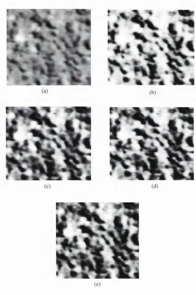
1.2 (a) and (b) for (0,1) displacement vector... 37 1.5 Illustration of an ultrasound kidney image region (a) unequalised

and equalised in (b) 256, (c) 64, (d) 32, and (e) 16 grey levels using the “equal probability quantizing” algorithm ... 38 1.6 The corresponding histograms of the images illustrated in Figure

1. 5... 39 1.7 3-D illustration of the co-occurrence m atrix of the images in Figures

1.5 (a) and (b) for (0,1) displacement vector... 41

C hapter 2

2.1 A neighbourhood configuration... 48

C hapter 3

(10)

3.3 Examples of MR images (a) femur image, (b) brain image... 83

3.4 Examples of CT images (a) brain image, (b) abdomen image. . . 86

C hapter 5

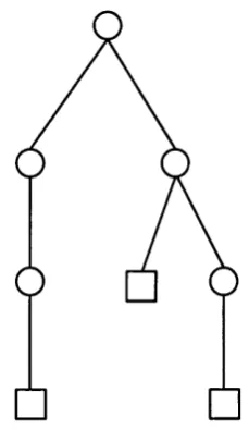
5.1 Example of the structure of a general tree T ... 109

5.2 Example of a binary tree... 110

5.3 Example of a full binary tree... 110

5.4 Example of a preorder and postorder traversal... 112

5.5 Example of a symmetrical traversal... 112

5.6 A complete full binary tree of depth 3...113

5.7 Construction of a complete full binary tree of depth 3 from a com plete full binary tree of depth 2 114 5.8 A worst case of a full binary tree having N =6 leaves... 115

5.9 Increasing the number of leaves without changing the depth of the tree... 116

5.10 Example of a full binary tree in the wide sense... 117

5.11 Illustration of the containment relation of the sets of the various types of binary trees... 117

5.12 A worst case full binary tree in the wide sense of depth 5... 118

5.13 Insertion of a new node (Case 1)... 123

5.14 Insertion of a new node (Case 2)...123

5.15 Insertion of a new node (Case 3)...124

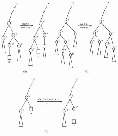
5.16 Illustration of the various cases of insertion in BB-tree... 131

5.17 Illustration of the various cases of insertion in BB-tree cont. . . . 132

5.18 Illustration of the various cases of insertion in BB-tree cont. . . . 134

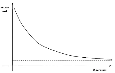
5.19 The cost curve of a perm utation rule and its asym ptote... 139

5.20 An example of an optimal search tree... 142

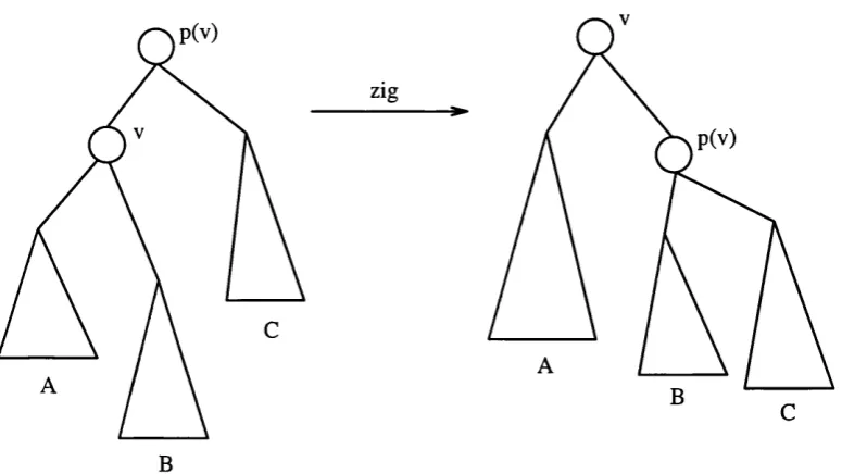
5.21 The zig case in splaying... 144

5.22 The zig-zig case in splaying... 144

5.23 The zig-zag case in splaying... 145

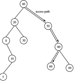
5.24 An example of a splay tree... 147

(11)

5.26 The structure of the tree after splaying at node 60... 148

C hapter 6

6.1 An example of the creation of the co-occurrence trees...154

6.2 An example of the creation of the co-occurrence trees cont... 155

6.3 An example of the list structures in the co-occurrence trees. . . . 156

6.4 Structure of a BB-tree node... 157

6.5 Structure of the semi-dynamic version... 160

6.6 Structure of the full-dynamic version... 161

C hapter 7

7.1 Semi-dynamic version with probability lists... 173

7.2 Full-dynamic version with probability lists... 174

7.3 An example of a BB-tree... 178

7.4 Plot of the worst case time cost of the access operation in the enhanced co-occurrence trees against the probability list length. . 183

C hapter 8

8.1 The zig case in top-down splaying... 196

8.2 The zig-zig case in top-down splaying...197

8.3 The zig-zag case in top-down splaying... 197

8.4 The final step in top-down splaying...198

C hapter 9

R ela tiv e p ercen tage red u ction in m em ory space for th e plain co-occurrence trees 9.1 Relative percentage reduction in memory space for the plain co occurrence trees; semi-dynamic version vs. co-occurrence m atrix. 207 9.2 Relative percentage reduction in memory space for the plain co occurrence trees; full-dynamic version vs. co-occurrence m atrix. . 208 9.3 Relative percentage reduction in memory space for the plain co

(12)

R ela tiv e p ercen tage reduction in m em ory space for th e enhanced co-occurrence trees (sta tic rule)

9.4 Relative percentage reduction in memory space for the enhanced co-occurrence trees (static rule); semi-dynamic version vs. co occurrence m atrix (a) Ng = 64, (b) Ng = 256, (c) Ng = 2048. . . 210 9.5 Relative percentage reduction in memory space for the enhanced

co-occurrence trees (static rule); full-dynamic version vs. co-occurrence m atrix (a) Ng = 64, (b) Ng = 256, (c) Ng = 2048... 211 9.6 Relative percentage reduction in memory space for the enhanced

co-occurrence trees (static rule); full-dynamic version vs. semi dynamic version (a) Ng = 64, (b) Ng = 256, (c) Ng = 2048. . . . 212

R ela tiv e p ercen tage reduction in m em ory space for th e enhan ced co-occurrence trees (m ove to front rule &

counter rule)

9.7 Relative percentage reduction in memory space for the enhanced co-occurrence trees (move to front and counter rule); semi-dynamic version vs. co-occurrence m atrix (a) Ng = 64, (b) Ng = 256, (c) Ng = 2048... 213 9.8 Relative percentage reduction in memory space for the enhanced

co-occurrence trees (move to front and counter rule); full-dynamic version vs. co-occurrence m atrix (a) Ng = 64, (b) Ng = 256, (c) Ng = 2048... 214 9.9 Relative percentage reduction in memory space for the enhanced

(13)

R ela tiv e p ercen tage red u ction in m em ory space for th e self-adjusting co-occurrence trees

9.10 Relative percentage reduction in memory space for the self-adjusting co-occurrence trees; semi-dynamic version vs. co-occurrence m a

trix ...216

9.11 Relative percentage reduction in memory space for the self-adjusting co-occurrence trees; full-dynamic version vs. co-occurrence m atrix. 217 9.12 Relative percentage reduction in memory space for the self-adjusting co-occurrence trees; full-dynamic version vs. semi-dynamic ver sion... 218

9.13 Relative percentage reduction in memory space using the self-adjusting co-occurrence trees instead of the plain co-occurrence trees (a) semi-dynamic version, (b) full-dynamic version... 219

T he analysed im age ty p e s 9.14 Asphalt image... 228

9.15 Grass image... 228

9.16 Fur image... 228

9.17 W ater image... 228

9.18 Weave image...228

9.19 Normal mammogram... 228

9.20 Abnormal mammogram... 229

9.21 Ultrasound heart image...229

9.22 Ultrasound kidney image... 229

9.23 Ultrasound liver image... 229

9.24 Ultrasound ovaries image... 229

(14)

T he effect o f d ynam ic range red u ction on th e te x tu r a l features

9.26 Examples of the percentage of the relative change in the values of the textural features of natural textures for various reduced grey level resolutions (a) asphalt image, (b) grass image, (c) fur image, (d) water image, (e) weave image... 230 9.27 Examples of the percentage of the relative change in the values of

the textural features of mammograms for various reduced grey level resolutions (a) normal mammogram, (b) abnormal mammogram. 232

C om p u tation al tim e resu lts for th e asphalt im ages

9.28 Plain co-occurrence trees (a) total time, (b) average time per re gion...237 9.29 Enhanced co-occurrence trees - static rule (a) semi-dynamic ver

sion, (b) full-dynamic version...237 9.30 Enhanced co-occurrence trees - move to front rule (a) semi-dynamic

version, (b) full-dynamic version... 238 9.31 Enhanced co-occurrence trees - counter rule (a) semi-dynamic ver

sion, (b) full-dynamic version...239 9.32 Self-adjusting co-occurrence trees (a) semi-dynamic version, (b)

full-dynamic version... 239

C om p u tation al tim e resu lts for th e grass im ages

9.33 Plain co-occurrence trees (a) total time, (b) average time per re gion...241 9.34 Enhanced co-occurrence trees - static rule (a) semi-dynamic ver

sion, (b) full-dynamic version... 243 9.37 Self-adjusting co-occurrence trees (a) semi-dynamic version, (b)

(15)

C om p u tation al tim e resu lts for th e fur im ages

9.38 Plain co-occurrence trees (a) total time, (b) average time per re gion... 245 9.39 Enhanced co-occurrence trees - static rule (a) semi-dynamic ver

sion, (b) full-dynamic version...247 9.42 Self-adjusting co-occurrence trees (a) semi-dynamic version, (b)

C om p u tation al tim e resu lts for th e w ater im ages

sion, (b) full-dynamic version... 249 9.45 Enhanced co-occurrence trees - move to front rule (a) semi-dynamic

sion, (b) full-dynamic version... 251 9.47 Self-adjusting co-occurrence trees (a) semi-dynamic version, (b)

C om p u tation al tim e resu lts for th e w eave im ages

sion, (b) full-dynamic version... 253 9.50 Enhanced co-occurrence trees - move to front rule (a) semi-dynamic

(16)

9.51 Enhanced co-occurrence trees - counter rule (a) semi-dynamic ver sion, (b) full-dynamic version... 255 9.52 Self-adjusting co-occurrence trees (a) semi-dynamic version, (b)

C o m p u tation al tim e resu lts for th e norm al m am m ogram s

9.53 Plain co-occurrence trees (a) total time, (b) average time per re gion...259 9.54 Enhanced co-occurrence trees (a) static rule, (b) move to front rule,

(c) counter rule... 259 9.55 Self-adjusting co-occurrence trees...260

C o m p u tation al tim e resu lts for th e u ltrasou n d heart im ages

C o m p u tation al tim e resu lts for th e ultrasou n d k idney im ages

(c) counter rule... 263 9.61 Self-adjusting co-occurrence....trees... 264

C o m p u ta tio n a l tim e results for th e u ltrasou n d liver im ages

(17)

9.63 Enhanced co-occurrence trees (a) static rule, (b) move to front rule,

(c) counter rule... 265

9.64 Self-adjusting co-occurrence trees... 266

C om p u tation al tim e resu lts for th e u ltrasound ovaries im ages 9.65 Plain co-occurrence trees (a) total time, (b) average time per re gion... 267

9.66 Enhanced co-occurrence trees (a) static rule, (b) move to front rule, (c) counter rule... 267

C om p u tation al tim e resu lts for th e u ltrasound spleen im ages 9.68 Plain co-occurrence trees (a) total time, (b) average time per re gion... 269

9.69 Enhanced co-occurrence trees (a) static rule, (b) move to front rule, (c) counter rule... 269

T he analysed im age ty p e s cont. 9.71 MR femur image...273

9.72 MR brain image (12 b it)...273

9.73 MR brain image (8 b it)...273

9.74 MR muscle image (12 b it)... 273

9.75 MR muscle image (15 b it)... 273

C om p u tation al tim e resu lts for th e M R bon e im ages 9.76 Plain co-occurrence trees (a) total time, (b) average time per re gion...274

(18)

C o m p u ta tio n a l tim e resu lts for th e 12 b it M R brain im ages

(c) counter rule... 276 9.81 Self-adjusting co-occurrence trees... 277

C o m p u ta tio n a l tim e resu lts for th e 8 b it M R brain im ages

C o m p u ta tio n a l tim e resu lts for th e 12 b it M R m uscle im ages

9.85 Plain co-occurrence trees (a) total time, (b) average time per re gion...280 9.86 Enhanced co-occurrence trees (a) move to front rule, (b) counter

rule (only the full-dynamic version; static rule was unable to give results)... 280 9.87 Self-adjusting co-occurrence trees...281

C o m p u ta tio n a l tim e resu lts for th e 15 b it M R m uscle im ages

9.88 Plain co-occurrence trees (a) total time, (b) average time per re gion...282 9.89 Enhanced co-occurrence trees (a) move to front rule, (b) counter

(19)

T h e analysed im age ty p e s cont.

9.91 CT liver image (32 x 32)... 286

9.92 CT liver image (16 x 16)...286

9.93 CT brain image (16 x 16)... 286

9.94 CT brain image (32 x 32)... 286

9.95 CT lung image... 286

C o m p u tation al tim e results for th e C T liver im ages (32 x 32 region size) 9.96 Plain co-occurrence trees (a) total time, (b) average time per re gion...287

9.97 Enhanced co-occurrence trees (a) move to front rule, (b) counter rule (only the full-dynamic version; static rule was unable to give results)... 287

9.98 Self-adjusting co-occurrence trees...288

C om p u ta tio n a l tim e results for th e C T liver im ages (16 x 16 region size) 9.99 Plain co-occurrence trees (a) total time, (b) average time per re gion...289

9.101 Self-adjusting co-occurrence trees...290

C om p u ta tio n a l tim e results for th e C T brain im ages (16 X 16 region size) 9.102 Plain co-occurrence trees (a) total time, (b) average time per region... 291

(20)

C o m p u tation al tim e resu lts for th e C T brain im ages (32 x 32 region size)

9.105 Plain co-occurrence trees (a) total time, (b) average time per region... 293 9.106 Enhanced co-occurrence trees (a) move to front rule, (b) counter

rule (only the full-dynamic version; static rule was unable to give results)...293 9.107 Self-adjusting co-occurrence trees...294

C om p u tation al tim e results for th e C T lung im ages

9.108 Plain co-occurrence trees (a) total time, (b) average time per region... 295 9.109 Enhanced co-occurrence trees (a) static rule, (b) move to front

rule, (c) counter rule... 295 9.110 Self-adjusting co-occurrence trees...296

T he eflfect o f dynam ic range red u ction on th e te x tu r a l features cont.

9.111 Examples of the percentage of the relative change in the values of the textural features of medical images for various reduced grey level resolutions (a) ultrasound kidney, (b) ultrasound spleen, (c) MR brain, (d) MR muscle, (e) CT liver, (f) CT lung...301 9.112 Example of the percentage of the relative change in the values

(21)

List o f Tables

C hapter 7

7.1 Optimal probability list length {Kopt) and worst time results from the simulation of the enhanced co-occurrence trees (ti) and the plain co-occurrence trees (^2) based on the model of page 181. . . 184

C hapter 9

9.1 Classification accuracy results from the performed experiments. . 226 9.2 Average sparsity of the co-occurrence matrices of the analysed data

(22)

Back Pocket

PU B L ISH ED PA PE R S

1. A. E. Svolos, C. A. Hutton, and A. Todd-Pokropek. Co-occurrence trees: A dynamic solution for texture feature extraction. In Proc. IE E E EM BS

18th Int. Conf. on Engineering in Medicine and Biology, pages 1142-1144, Amsterdam, The Netherlands, 1996.

2. A. E. Svolos and A. Todd-Pokropek. An evaluation of a number of tech niques for decreasing the computational complexity of texture feature ex traction through an application to ultrasonic image analysis. In Proc. IEE E EM BS 19th Int. Conf. on Engineering in Medicine and Biology, pages 601- 604, Chicago, IL, 1997.

3. A. E. Svolos and A. Todd-Pokropek. Self-adjusting binary search trees: An investigation of their space and time efficiency in texture analysis of magnetic resonance images using the spatial grey level dependence method. In Proc. SP IE Medical Imaging Int. Conf.: Image Processing, pages 220- 231, San Diego, CA, 1998.

(23)

C hapter 1

In trod u ction

1.1 Texture — A n essential im age feature

Texture is a fundamental feature th at can be used in the analysis of images in several ways, e.g. in the classification of medical images into normal and abnor mal tissue, in the segmentation of scenes into distinct objects and regions, and in the estimation of the three-dimensional orientation of a surface. Texture has long been recognised as a key to human perception. Therefore, it has been ex tensively employed in computer vision tasks. Its importance has been proved for many types of images ranging from multi-spectral remote sensed aerial and satel lite d a ta to biomedical images. In particular, in medical image analysis texture has been successfully employed for tissue characterisation, i.e. the determ ina tion of tissue type (normal or pathological) and further classification of tissue pathology (see [97]), in many cases. Texture analysis has been shown to increase the level of diagnostic information extracted from various image types of most medical imaging modalities and to quantitatively characterise differences in tissue imperceptible by human observers.

(24)

the above references distinguish between tone and texture in grey level images. Tone is equivalent to grey level assigned to each pixel in an image.

Texture can be considered to be decomposed into two constituents, namely the tonal primitives and the placement rules. A tonal primitive is a maximally connected set of pixels (a region) having a given tonal property, such as a range of grey levels. This region can be described in terms of its area and shape. Tonal primitives can be geometrical objects, such as line segments or closed polygons. On the other hand, the primitive placement rules describe the spatial dependence among the primitives in the texture. Therefore, an image texture can be described by the number and types of its primitives as well as the spatial organisation of its primitives determined by the placement rules. This organisation may be random or determined by the spatial dependence of one primitive on a neighbouring prim itive (second order), or, in general, on n — 1 neighbouring primitives (nth order). Another way to define texture is by considering it as a global pattern resulting from the repetition, either deterministically or randomly, of local sub-patterns.

One im portant aspect of texture description is its scale dependence, accord ing to [144]. T hat means th a t texture primitives can be defined in more than one hierarchical level. At different scales different textures may arise, coarser or finer. Coarseness is one of the properties th a t qualitatively describe texture. O ther such properties are smoothness, granulation, randomness, etc. According to [61], the two major properties of a texture are its coarseness and directionality. Each of these properties translates into some property of the tonal primitives and the spatial dependence among them. For example, a fine texture results if the tonal primitives are small and there is a large variation between neighbouring primitives. On the other hand, if the tonal primitives are larger (they consist of a larger number of pixels) a coarse texture arises. In any case, the fine/coarse texture property depends on scale.

(25)

ships and are usually sufficiently described by means of the frequency of co occurrence of pairs of texture primitives in some spatial relationship. Therefore, both primitives and primitive placement rules are necessary for the characterisa tion of such textures.

The main problem in texture analysis is th a t real textures are extremely diffi cult to define m athematically and therefore, get analysed by machines, although it is a quite easy task for human beings to recognise and describe them in em pirical terms. It is this lack of definition th a t makes autom atic description or recognition of textures a very complex and as yet an unsolved problem.

1.2 Texture analysis

According to [61], two major texture analysis methods exist: statistical and syn tactic or structural. Statistical methods employ scalar measurements (features) computed from the image data, which characterise the analysed texture. In this context, texture is described by a set of statistics extracted from a large ensemble of local picture properties. First order statistics, such as the grey level mean and the grey level variance, have been employed in the classification of a limited set of textures. Second order statistics, such as those computed in the SGLDM, have been widely used in texture analysis. Higher order statistics can also be measured. The features extracted by the statistical methods usually measure textural characteristics, such as coarseness, contrast, and directionality.

(26)

A primitive is characterised by a list of attributes, such as the average grey level, the area of the primitive region, and its shape. Primitive spatial relation ships are usually described by means of a grammar which represents the rules for building a texture from a set of primitives. W ithin this context, there is a one to one correspondence between textures and formal languages. Symbols represent ing the primitives comprise the alphabet. Transformation rules th a t represent the spatial relationships between primitives, apply to the symbols of the alphabet to generate the texture. A tree grammar is commonly used to represent these placement rules. This texture description method is best for regularly structured textures. Real textures, though, are most often irregular, in the sense th a t struc tural errors, distortions, or even structural variations, frequently happen in them. Thus, to make syntactic description of real textures feasible, variable rules must be incorporated into the description grammars and non-deterministic or stochas tic grammars must be employed (see [55]).

Several ways have been devised for the extraction of primitive descriptions and placement rules from a given texture. In [78], [107], the traditional Fourier spectrum of an image was employed for this purpose. In [161], a texture prim itive was assumed to be a region of homogeneous grey level. The problem of extracting primitives from a given texture was therefore equivalent to the prob lem of segmenting the image into homogeneous regions. The placement rules were computed from the relative positions of the centroids of the extracted primitives. In [171], the structural texture description algorithm first computed the edge map of the given texture and afterwards, it extracted the texture primitives grouped by type, employing this map. Once the primitives were isolated, it employed the relative positions of the centroids of nearest-neighbour primitives to produce a set of placement rules.

1.3 T exture classification and segm entation

(27)

class (sample labelling). For example, in medical image processing the classes may be normal and abnormal breast tissue and the goal, the determ ination of whether a given digital X-ray breast image (mammogram) belongs to the first or the second class. There are three general methods for solving the above problem:

1. statistical classification,

2. syntactic or structural classification, 3. neural network classification.

Syntactic classification is based on some sort of description of the structure of the texture in each image region (see Section 1.2). According to the actual type of structural description employed, a different classification approach is followed. In [171], a symbolic representation was constructed from each texture sample and a decision tree utilised this information to classify the samples. In [161], the prop erties of the primitives and primitive placement rules of each texture region were computed and compared with the corresponding properties of models describing texture classes. Each texture sample was assigned to the class the model of which was closest to the properties of the sample. In [55], the unknown texture was rep resented by a string of symbols and a method known as parsing (see [133]) was used to determine the grammar th at could produce this string and consequently its texture class. Syntactic description is suitable to the analysis and classification of textures exhibiting a more regular structure. For this reason, syntactic texture description methods have seen limited use in real texture analysis applications, especially in medical image processing. Therefore, we will not present them in more detail.

Neural network classification is based on artificial neural networks, which are relatively new computing systems whose architecture is made of a large number of interconnected simple processing elements called nodes. The input of each node is the weighted sum of the output of all the nodes to which it is connected. Its output value is, in general, a non-linear function of this sum. This function is referred to as the activation function of the nodes.

(28)

called neurons. The basis of these computations is a small number of serial steps, each of which is massively parallel employing a vast number of simple processing cells which are locally connected. They allow the real time processing of complex information. Neural networks are, in a sense, a non-algorithmic, black box approach. This black box is trained in order to learn the correct response (e.g. correct classification) for each of the training samples. From this point, it is an attractive approach, since it minimises the required amount of a priori

knowledge of the properties of the d ata and detailed knowledge of the internal system operation. After training, it is hoped th a t the internal structure has been self-organised to enable the correct response for new, yet similar, data, based on the “experience” gained from the training set.

One of the most popular artificial neural networks is the back propagation neural network. Its training consists in finding a mapping between the set of input values and the set of output values. This mapping is accomplished by adjusting the weights using a learning algorithm, such as the generalised delta rule (see [133]). After the weights are adjusted on the training set, their values become fixed and the neural network can be employed for the classification of unknown samples.

(29)

Test samples Training samples (labelled) Texture class Processed Feature

samples measurements decisions

Non-parametric Parametric Processed Feature samples measurements Classifier Preprocessor Preprocessor Parameter Estimator Extractor Feature Extractor Feature

Figure 1.1: A typical statistical texture classification system.

The above studies showed th at the neural network approach is a potential im mediate com petitor against statistical classification, but further evaluation of its performance needs to be carried out, especially in medical image analysis.

Statistical classification is based on characteristic measurements (features) extracted from the analysed textural region. Usually, these scalar measurements are organised in a vector form (feature vector), which characterises the analysed texture. A block diagram outlining a typical statistical texture classification system, modified from [170], is shown in Figure 1.1. Actually, the illustrated system is a supervised classification system. This is the most common system in texture classification.

There are two broad categories of classification strategies: supervised and unsupervised. In supervised classification, the texture classes are known a priori

(30)

the problem of unsupervised classification is much more difficult.

The classifiers are further categorised into param etric and non-parametric. In param etric classification, the parameters of the class-conditional sample density functions must first be determined from the training data, given the form of these functions (e.g. Gaussian or uniform). In practice, we may not be able to determine a specific form. In this case, non-parametric classification must be employed, where the training samples are directly used for the classification. The performance of the classifiers is usually determined by the percentage of samples correctly classified (classification accuracy).

One of the most interesting supervised non-parametric classifiers is the

k-nearest neighbour classifier. This is a simple classifier, which is widely used, especially when the underlying class-conditional probability distributions are un known. It classifies a given test sample by assigning it the label th a t most fre quently encountered among the k nearest to it training samples (see [48]). The Euclidean metric ([133]) is commonly used for the computation of the distance between the test sample and each training sample. The leave-one-out method ([56]) is most often used for the estimation of the classification accuracy of this classifier for a given classification problem. According to this method, one sample from the set of labelled samples is excluded, the classifier is trained on the remain ing samples (training set), and subsequently, the excluded sample is tested using the classifier (test sample). This operation is repeated for each sample in the set of labelled samples. Then, the number of correctly classified samples is counted in order to estimate the classification accuracy. According to [29], [56], [65], the

leave-one-out method is widely used, when the number of available samples for each class is relatively small.

(31)

constituent parts of the classification system, significantly increasing the time and memory space of the whole texture classification process. Reducing the dynamic range of the analysed textures is one way to keep these requirements tolerable. However, as we will see in the next chapters, this reduction may lead to significant information loss which can be vital, especially in medical image analysis. There fore, efficient algorithms, in terms of computational time and memory space, must be devised for the feature extraction stage. This is also justified by the fact th at this stage is an essential part, not only of a texture classification system, but also of a texture segmentation system and in general, of any texture analysis system.

Developing time and space efficient algorithms will help not only to speed up the whole process, but also to minimise grey level reduction, possibly allowing for more useful information to flow into the feature extractor, more descriptive texture features to be computed and consequently, better classification accuracy to be achieved. In this thesis, a number of algorithms for the feature extraction stage, which show efficiency in both time and space, are proposed and evaluated for one of the best and most widely employed texture analysis methods, namely the Spatial Grey Level Dependence Method (SGLDM).

Finally, we will say a few words about the texture segmentation problem. This problem involves the accurate partitioning of an image into differently textured regions (textures). Alternatively, texture segmentation can be viewed as the problem of accurately delineating the borders between different textures in an image. Two types of methodologies are widely employed to solve the general image segmentation problem ([26]). The first one is the region growing m ethod ology, which starts from small regions with certain properties and expands them as long as their properties are not violated. The other one is the edge detection, which searches for parts of the image where a transition occurs from one region to another region having different properties. The interested reader should refer to one of the many surveys of texture segmentation techniques ([61], [74], [126], [173]).

(32)

teeth (see Section 3.2). In [109], digital chest radiographs were segmented into various regions, such as the heart and the lungs, based on texture features ex tracted from local neighbourhoods around each pixel (see Section 3.2). Fortin et al. ([53]) attem pted to segment Magnetic Resonance (MR) cardiac images into the ventricular walls and the ventricular blood pools (see Section 3.4). In [99], MR brain images were segmented into white m atter, grey m atter, and CSF (Cere- broSpinal Fluid) (see Section 3.4). The same segmentation (white and grey m at ter only) was attem pted in [19], analysing Computed Tomography (CT) images of the brain (see Section 3.5). Finally, in [22] electron micrograph images of cells were segmented into the various parts of the nucleus, employing a number of texture analysis methods (see Section 3.6).

1.4 Equal probability quantising

Texture samples usually pass through a pre-processing stage (the first stage in the texture classification pipeline in Figure 1.1) before feature extraction. This stage performs functions such as normalisation, enhancement, or noise cleaning on the image. However, the pre-processor in texture analysis serves two main purposes. First, it normalises the data to eliminate undesirable effects, such as variations in illumination. Second, it requantises the data in a known fashion.

The normalisation usually consists in modifying the grey levels of the original image data, so th a t the resulting image histogram is uniformly shaped (histogram equalisation). In this way, all first order statistical information, such as sample mean and sample variance, is lost. The justification for performing this step is th a t first order statistics can be directly affected by factors such as variations in illum ination and thus, histogram equalisation (normalisation) serves to remove these undesirable effects. Also, research in visual perception indicated th a t tex ture is characterised by higher order spatial statistics ([57], [80], [81]).

(33)

due to the large time and space requirements of the co-occurrence m atrix. Grey level reduction can also be justified when the initial image contains noise which may adversely affect texture analysis, or redundant information (redundancy here refers to any information not necessary to achieve a certain level of texture dis crimination).

In the experiments performed in this thesis, equal probability quantisation was employed for normalising the histograms of the analysed textures. The basic idea behind the “equal probability quantizing” algorithm is the step by step approximation of the cumulative probability function of a uniform distribution, based on the estimated cumulative probability function of the original texture. A detailed description and analysis of this algorithm can be found in [65].

Equal probability quantising has been used for the normalisation of various texture types by many researchers ([61]). In [101], it was employed for pre processing natural textures, prior to texture analysis. Shanmugan et al. ([136]) employed equal probability quantising for normalising radar images illustrating various geological formations. Similarly, in [58] and [176] it was employed for flat tening the histogram of satellite images showing geological terrain types. In [64], equal probability quantising was employed for the normalisation of photomicro graph images of various sandstone types.

(34)

reduction. However, as far as we know, there is no study which clearly shows th at this algorithm is the best pre-processing technique for all medical image types. Additionally, the normalisation (histogram equalisation) of medical images prior to texture analysis may not be appropriate in all cases.

We will present two examples th at show the effectiveness of the “equal prob ability quantizing” algorithm. In the first example, a natural texture image illus trating asphalt was normalised. The image had a size of 512 x 512 and its initial dynamic range was 8 bits (256 grey levels). From this image, a region of size 64 X 64 was extracted and normalised in 256, 64, 32, and 16 grey levels. In Fig

ures 1.2 (a)-(e), the unequalised image region and the equalised image regions for the above dynamic ranges are illustrated. In addition, in Figures 1.3 (a)-(e) the corresponding histograms are shown. These figures clearly show the equalisation effect of the “equal probability quantizing” algorithm, which becomes stronger as the number of grey levels becomes smaller, since the uniform distribution is better approximated. Finally, in Figure 1.4 a 3-D illustration of the co-occurrence m atrix (2-D histogram) for (0,1) displacement vector (see Section 4.1) is shown before normalisation and after normalisation for the initial dynamic range. From these figures, it is clear th at the grey level pairs are more spread out in the nor malised region, as a result of the uniform distribution approximation in first order statistics (1-D histogram).

(35)

(a)

t

s

(c) (d)

(e)

Figure 1.2: Illustration of an asphalt image region (a) unequalised and equalised in (b) 256, (c) 64, (d) 32, and (e) 16 grey levels using the

(36)

median = 163 116

Count

Pixel value histogram (a)

median = 94 116

Count

Pixel value histogram 133

(b)

Count

median = 30

(37)

median = 16 198

Count

300

Count

Pixel value histogram

(d)

median = 8

Pixel value histogram (e)

(38)

(a)

(b)

(39)

(a) (b)

(c) _(d)

###

(e)

Figure 1.5: Illustration of an ultrasound kidney image region (a) unequalised and equalised in (b) 256, (c) 64, (d) 32, and (e) 16 grey levels

(40)

median = 67 41

Count

I

J

Li«_u __ |_

i histog (a)

median = 118 41

Count

_________ I

Pixel value histogram 141

(b)

median = 40 41

Count

Pixel value histogram 63

(41)

median = 15

Count

(d)

median = 8

Count

Pixel value histogram (e)

(42)

(a)

(b)

(43)

1.5 C ontributions and general organisation of

th e th esis

In this thesis, three novel approaches which are based on dynamic binary trees to organise the textural information extracted from an image region by the SGLDM, are presented and evaluated both theoretically and through their application to the analysis of natural textures and medical images of various modalities. Their novelty is based on their ability to eliminate the redundant information stored in the co-occurrence m atrix in the form of zero entries, due to their dependency only on the number of distinct grey levels in the analysed local region. The zero estim ated co-occurrence probabilities contribute nothing to the com putation of the textural features. The proposed approaches are shown to provide efficiency in both storage requirements and computational time compared to the co-occurrence m atrix, especially in the analysis of images employing their full dynamic range. Two experiments involving the classification of clinical and non-clinical image d a ta are performed, which clearly show the benefit of analysing images using SGLDM, w ithout reducing their grey level range.

(44)

C hapter 2

T exture analysis m eth od s

In the last 25 years, a large number of texture analysis methods have been pro posed in numerous papers. A detailed presentation of all of these algorithms is beyond the scope of this thesis. The interested reader should refer to one of the many excellent surveys ([38], [61], [63], [108], [126], [173]). In this chapter, we review the most referred in texture analysis literature and the most recently de vised texture characterisation methods, with emphasis on those being employed in medical image analysis. The Spatial Grey Level Dependence Method (SGLDM) is presented in a separate chapter (Ghapter 4).

2.1 Grey level difference m ethod

The grey level difference method has been widely used in texture analysis appli cations, especially in remote sensing ([47], [94], [95], [174]). This method is based on statistics computed from a grey level difference histogram ([38], [176]). A grey level difference histogram gives the frequency of occurrence of pairs of pixels sep arated by a displacement vector d and whose grey levels differ by a fixed amount

k. It is defined as:

H{k]d) = #{{{xi , yi), {x2, y2)) ■ \I{xi,yi) - I{x2,y2)\ = k A

X2 = Xi-\-dx A y2 = y \ + dy} (2.1)

(45)

this histogram can be intuitively related to texture structure. If the displacement vector d is small, high frequency values for large differences (large k) indicate a fine texture, whereas high frequency values for small differences (small k) indicate a coarse texture.

Usually, the normalised grey level difference histogram is computed, th a t is,

H{k]d) is divided by the total number of pairs of pixels separated by the dis placement vector d. One statistic th at has been used as a texture feature is the mean statistic defined as:

M E A N = y ; fc • d) (2.2)

k

(see [38]). Other features th a t can be extracted from the normalised grey level difference histogram include contrast, angular second moment, entropy ([176]) and inverse difference moment ([33]).

2.2 Grey level run length m ethod

A grey level run length primitive (or simply grey level run) is a maximal collinear connected set of pixels having the same grey level. Grey level runs are charac terised by the grey level of the run, the length of the run, and the direction of the run. Their intuitive relation to the structure of a texture is th a t a coarse texture is expected to give relatively long runs more often, whereas a fine texture should primarily contain short runs.

The grey level run length method is based on grey level runs. It was intro duced by Galloway ([58]). Galloway estimated the joint probability p(z, j; i9) of runs of grey level i and length j from a textured region for various directions d.

From this estimated joint probability she extracted five texture features, namely short run emphasis, long run emphasis, grey level non-uniformity, run length non uniformity, and image fraction in runs. This texture analysis m ethod has been employed especially in remote sensed data analysis ([1], [9]).

(46)

• it is very sensitive to noise

• it does not capture the very im portant information contained in the second order probabilities of the form p(z, j) , i ^ j , where j are grey levels of pixels at a specific interpixel distance and orientation.

2.3 T exture description using stoch astic m odels

Texture description methods based on stochastic models consider textures as realisations of stochastic processes. These models assume th a t a pixel has some kind of dependence on its neighbourhood. This can be a linear dependence (e.g. autoregressive models) or a conditional probability (e.g. Markov random field model). The param eters of the model are estimated from the analysed region and used as texture descriptors. A number of stochastic models have been used in the past for texture description.

In [21], an image region I(x, y) is decomposed into a series of grey level planes defined as:

1 , i î l ( x , y ) = g fg{^: y) —

0 , M I { x , y ) i - g ^

for p = 0 , 1 , . . . , Ag — 1, where Ng is the number of grey levels in the analysed texture. The texture is characterised by the probability distribution of the pixel counts Xg, where Xg = fg{^^ v)- Actually, Xg is the number of pixels th at belong to grey level plane g. A parametric stochastic model is used for describing the probability distribution oî Xg, g = 0 , 1 , Ng — 1, for the given texture. If the pixels in each grey level plane are assumed to be distributed randomly, the pixel counts can be described by a Poisson distribution. In some cases, however, this assumption is not valid due to local clustering of points.

One class of models th a t are capable of describing clustered d ata includes mixtures of Poisson distributions. For a mixture of k different Poisson densities the model is described by:

= (2-4)

(47)

where 7t^^\ j = 1, . . . , k are the relative frequencies of the Poisson densities {x)

with parameters i.e.

M)

The authors claim th at mixture models of 2 and 3 Poisson densities give very satisfactory results in texture classification.

Markov random fields (MRF) have been widely used as texture models. In this context, a Markov random field considers the grey level of a pixel to be dependent on the grey levels of pixels in some neighbourhood. Actually, this is always the case in reality unless the image is simply random noise. Let L be a lattice of size N x N and I{x, y) denote the grey level at pixel (x, y) on lattice L.

We can relabel 7(x, y) to be 7(z), z = 1 , 2 ,. .. , M where M = N'^. Point j is said to be a neighbour of point i if the conditional probability

|/{1), 7 ( 2 ) ...., 7(i - 1). 7(i + 1 ) , . . . , 7(M ))

depends on 7(j). The above relation does not imply th at the neighbours of a point are necessarily close in terms of distance, although this is the usual case. A colouring X of lattice L with Ng levels is a function from the points of L to the set { 0 ,1 ,..., Ag — 1}. According to [36], a Markov random field is described by a joint probability density on the set of all possible colourings X of the lattice L

which satisfies the following conditions:

• positivity: P { X ) > 0, for all X,

• Markovianity: P { X { i ) \ X { j ) for all j G { 1 ,..., A7}, j ^ i} = P { X { i ) \ X { j ) for all j th a t belong to a neighbourhood of z},

• homogeneity: the above conditional probability depends only on the con figuration of the chosen neighbourhood and is translation invariant.

In [36], the so-called autobinomial model is utilised (see also [14]). In this model, the conditional probability P { X { i ) = k\ X{ j ) for all j in neighbourhood} where A; G { 0 ,1 ,..., Ag —1}, is binomial with param eter ’â{T) = and number

(48)

the Markov random field in turn depends on the neighbourhood (see [36]). From the above, the conditional probability P { X { i ) = k\ neighbours} can be w ritten as:

T \ k

P { X { i ) = k \ T } =

A: _/ 1 +

Na —k — 1

(2.6)

Cross et al. ([36]) claimed th at texture properties, such as directionality and coarseness, can all be refiected in the param eter values of the above model. The Markov random field model is more appropriate for microtextures. Textures showing regularity and inhomogeneous textures do not seem to fit very well. Also, large image regions are required to get good param eter estimates.

In [27], a texture description method was proposed which employs the corre lation coefficients between pixel pairs {I{x,y), I {x dx,y dy)), where {dx,dy)

represents the displacement vector. It holds th at 0 < max(dxj dy) < d, where d

is a small number. More specifically, two pixels far away from each other are as sumed to be uncorrelated. The texture is modelled by a two-dimensional second order discrete (homogeneous) Gaussian random field. Therefore, the second order probabilities p{k,l-,dx,dy) = Prob{I{x, y) = k, I{x -h dx,y P dy) = /} are char acterised by the mean vector m and covariance m atrix V . Since the underlying random field is stationary (homogeneous), m = (m, m), where m is the expected value of the grey level of a pixel (average image brightness). The covariance m atrix V is defined as:

V = = cr^ •

1 Pdx dy

Pdx dy 1

(2.7)

where is the variance of grey level and pd^dy the correlation coefficient for the displacement vector {dx,dy). These coefficients describe the spatial dependencies of pairs of pixels (second order statistics) and can be used as texture features.

(49)

(x,y) (x+l,y)

( x ,y + l ) ( x + l , y + l )

Figure 2.1: A neighbourhood configuration.

I{x^y), —oo < x , y < oo. This image is obtained by repeating the corresponding finite image an infinite number of times, using an appropriate repetition formula. Then, I { x , y ) is assumed to be generated from the random field described by the autoregressive equation:

n y—

■ / ( % , * ) = y P - u { x , y ) (2.8) k=l

where {{xk,yk)}k=i..n defines the effective neighbourhood of infiuence for pixel

{x, y). For example, a possible neighbourhood is {(a; — 1,2/), (x, 2/ — 1), (a; + 1 ,2/), (a:,y + 1), (a: + 1,2/ + 1)} (see Figure 2.1). { u ( x , y ) } _ ^ ^ ^ y ^ ^ is a sequence of Gaussian independent identically distributed (i.i.d.) random variables with zero mean and unit variance. The texture is described by the estim ated param eters

{6, /3), where 0 = (i?i,. . . ,

2.4 T exture analysis based on local linear trans

forms

(50)

first defined, which correspond to features such as edge, spot, and wave, e.g.:

: — 1 0 1

: —1 2 —1

Ws : - 1 2 0 - 2 1

The index of the above vectors indicates their size.

The 1 x 3 vectors form a basis for the larger vector sets. Each 1 x 5 vector can be generated by convolving two 1 x 3 vectors. A set of 1 x 7 vectors can be generated by convolving 1 x 3 and 1 x 5 vectors, or by twice convolving 1 x 3 vectors. Similarly, by convolving a vertical vector mask with a horizontal vector mask, m atrix (two-dimensional) masks are formed, e.g.

1 0 - 1

SzE^ : - 2 0 2

1 0 - 1

The names indicate the vector masks used for their generation. In a similar manner, we can get 5 x 5 and 7 x 7 masks.

The most im portant property of the above two-dimensional masks is th a t they are separable, so only one-dimensional convolution operations with the image are required, which are computationally cheap. After the image is convolved with the appropriate mask, it is processed with a non-linear local texture energy filter, such as a moving-window average of the absolute filtered image values. Texture is characterised by the texture energy values at each pixel location resulting from the application of several convolution masks.

2.5 T exture analysis based on fractals

Fractals provide a m athem atical framework to study the irregular complex shapes found in nature. According to Mandelbrot ([105]), one im portant criterion for a bounded set A in Euclidean n-space to be a fractal set is its self-similarity. A

(51)

copies of itself, each of which has been scaled down by a ratio r in all co-ordinates. The fractal or similarity dimension D of A is given by the relation: 1 = N{r) • or equivalently D = . The natural fractal surfaces, such as the textural surfaces, do not in general possess this deterministic self-similarity. Instead, they exhibit statistical self-similarity, th at is, they are composed of N{r) distinct sub sets each of which is scaled down by a ratio r and is identical in all statistical respects to the original. The fractal dimension of these surfaces is also given by the above relations.

Pentland ([122]) presented evidence th a t most natural surfaces are spatially isotropic fractals and th at intensity images of these surfaces are also fractals. Actually, this work provided the foundation for the use of features derived from fractal models (e.g. fractal dimension) in image analysis. More importantly, Pentland introduced fractal based texture analysis by showing th at there exists a correlation between texture coarseness and the fractal dimension of a texture. He proposed fractal functions as texture models and the fractal dimension as the texture feature. The fractal dimension has been shown to correlate with the intuitive roughness of a texture. A small value of fractal dimension D indicates a sm ooth texture, whereas a large value of D indicates a rough texture. There are various methods for estimating the fractal dimension from a textured region (see [85], [131]).

O ther fractal parameters have also been employed for texture characterisation. In [102], the H param eter was used. H was related directly to D, the fractal dimension, hy D = 2 — H. Four values of H in each region of a textured image were estim ated, one for each principal direction (horizontal, vertical, and two diagonals). Then, a composite average H was computed by averaging the H

(52)

Another im portant fractal parameter, which has been used for texture de scription is lacunarity. Given a fractal set A, let p(m) be the probability th at there are m points within a box of size L centred about an arbitrary point of A.

It holds th a t J2m=iP('^) = 1, where K is the number of possible points within the box. The lacunarity can be defined as follows:

13.9)

where M = Em=i ^ ' p (W and M2 = J2m=i Lacunarity is small when

the texture is dense (fine) and large when the texture is coarse. Actually, this param eter was introduced to describe fractal surfaces having the same fractal dimension but different appearances (see [105]). According to [85], the fractal dimension alone is not sufficient for the description of natural textures. The authors claimed th a t both lacunarity and fractal dimension need to be employed for this purpose.

Space and time efficient data structures in texture feature extraction