Magnetic Otto engine for an electron in a quantum
dot: classical and quantum approach
Francisco J. Peña1*, O. Negrete1, G. Alvarado Barrios3,4, D. Zambrano1, Alejandro González1, A. S. Nunez2, Pedro A. Orellana1and Patricio Vargas1,4 ID
1 Departamento de Física, Universidad Técnica Federico Santa María, Casilla 110 V, Valparaíso, Chile;
[email protected] (O. N.); [email protected] (D. Z.); [email protected] (A.G.); [email protected] (P.A.O.); [email protected] (P.V.)
2 Departamento de Física, Facultad de Ciencias Físicas y Matemáticas, Universidad de Chile, Casilla 487-3,
Chile; [email protected]
3 Departemento de Física, Universidad de Santiago de Chile (USACH), Avenida Ecuador 3493, 9170124, Chile;
4 Centro para el Desarrollo de la Nanociencia y la Nanotecnología, Santiago, Chile
* Correspondence: [email protected] ; [email protected]
Version January 9, 2019 submitted to
Abstract:We study the performance of a classical and quantum magnetic Otto cycle with a quantum 1
dot as a working substance using the Fock-Darwin model with the inclusion of the Zeeman interaction. 2
Modulating an external/perpendicular magnetic field, we found in the classical approach an 3
oscillating behavior in the total work that is not perceptible under the quantum formulation. Also, we 4
compare the work and efficiency of this system for different regions of the Entropy,S(T,B), diagram 5
where we found that the quantum version of this engine always shows a reduced performance in 6
comparison to his classical counterpart. 7
Keywords:Magnetic cycle; Quantum Otto cycle; Quantum Thermodynamics. 8
1. Introduction 9
The study of quantum heat engines (QHEs) [1] is focused on the search and design of efficient 10
nanoscale devices operating with a quantum working substance. These devices are characterized 11
by their working substance, the thermodynamic cycle of operation, and the dynamics that govern 12
the cycle [2–26]. Amongst the cycles in which the engine may operate, the Carnot and Otto cycles 13
have received increasing attention. In particular, the quantum Otto cycle has been considered for 14
various working substances such as, spin-1/2 systems [27,28], harmonic oscillators [29], among others. 15
Furthermore, the quantum Otto cycle has been experimentally realized in trapped-ions [30]. 16
Previous studies of the quantum Otto cycle embedding working substances with magnetic 17
properties have highlighted the role of degeneracy in the energy spectrum on the performance of the 18
engine. [31–33]. In this same framework, we highlight the work of Mehta and Ramandeep [34], who 19
worked on a quantum Otto engine in the presence of level degeneracy, finding an enhancement of 20
work and efficiency for two-level particles with a degeneracy in the excited state. Also, Azimi et al. 21
presented the study of a quantum Otto engine operating with a working substance of a single phase 22
multiferroicLiCu2O2tunable by external electromagnetic fields [35] and is extended by Chotorlishvili 23
et al. [36] under the implementation of shortcuts to adiabaticity, finding a reasonable output power for 24
the proposed machine. Recently an electron confined inside a semiconductor quantum dot has been 25
studied in the context of an isoenergetic cycle [37]. This system is externally driven by an external 26
magnetic field finding that in the high magnetic field regime the efficiency achieves the asymptotic 27
limit in agreement with results previously reported in the literature for mechanically driven quantum 28
engines. On the other hand, the classical version of the Otto cycle consists of two isochoric processes 29
and two adiabatic processes. If the working substance is a classical ideal gas, the first approximation 30
for efficiency depends on the quotient of the temperatures in the first adiabatic compression. This 31
expression is reduced with the specific condition along the adiabatic trajectory for this kind of gas, 32
given byTVγ−1= cnt., whereγ= C
P/CV obtaining the expressionη=1−rγ1−1, whereris called 33
“compression ratio" that is defined asV1/V2(withV1>V2). For magnetic substances, like diamagnetic 34
systems, the condition obtained for the adiabatic stroke, in general, is not trivial. This is due to the 35
complexity of the energy spectra as a function of the external magnetic field for this kind of systems. 36
This is later reflected in the partition function from which the thermodynamic quantities under study 37
are obtained. In particular, it is interesting the comparison of the classical and quantum approaches for 38
the same magnetic working substance and establish the conditions for each case appropriately. Besides, 39
physically it is nowadays possible to confine electrons in 2D. For instance, quantum confinement can 40
be achieved in semiconductor hererojunctions, such as GaAs and AlGaAs. AtT=300 K, the band gap 41
of GaAs is 1.43eVwhile it is 1.79 eV for AlxGa1-xAs (x=0.3). Thus, the electrons in GaAs are confined 42
in a 1-D potential well of length L in the Z-direction. Therefore, electrons are trapped in 2D space, 43
where a magnetic field along Z-axis can be applied [38]. 44
Therefore, in this work, we study the performance of a multi-level classical and quantum Otto 45
cycle where the working substance comprises a nanosized quantum dot under a controllable external 46
magnetic field. This system is described by the Fock-Darwin model [39,40] that represents an accurate 47
model for a semiconductor quantum dot. 48
2. Model 49
Let us consider an system given by a electron in the presence of a parabolic potential and external 50
magnetic fieldB. The Hamiltonian which describes the system is given by 51
ˆ
H= 1
2m∗(p+eA) 2
+UD(x,y), (1)
wherem∗is the effective electron mass,Ais the total vector potential, and the termUD(x,y)is given 52
by 53
UD(x,y) = 1 2m
∗ ω02
x2+y2, (2)
which corresponds to an attractive potential describing the effect of the dot on the electron. The 54
quantity ω0is the parabolic trap frequency and can be controlled geometrically. If we consider a 55
constant perpendicular magnetic field in the form 56
B=Bzˆ, (3)
and the use of the vector potentialAin the symmetric gauge (i. e.A= B2(−y,x, 0)), the solution of 57
the eigenvalues of the Schrödinger equation are given by 58
Enm =¯hΩ(2n+|m|+1) +1
2¯hωcm. (4)
where, ωc = meB∗ is the cyclotron frequency, n, mare the radial and magnetic quantum numbers
59
(n=0,1,2,... andm=−∞,...,+∞).Ωit is known as the effective frequency of the system corresponding to 60
Ω=ω0 1+
ωc 2ω0
2!
1 2
. (5)
Notice that when the parameterω0→0, the energy levels of Equation (4), take the usual form of the 61
0 1 2 3 4 5 6 0 5 10 15 20 25 30
ωc/2ω0
E
/
¯
h
ω0
(a)σ= –1 n = 0 n = 1 n = 2 n = 3 n = 4 n = 5 n = 6
0 1 2 3 4 5 6 0 5 10 15 20 25 30
ωc/2ω0
E
/
¯
h
ω0
(b)σ= +1 n = 0 n = 1 n = 2 n = 3 n = 4 n = 5 n = 6
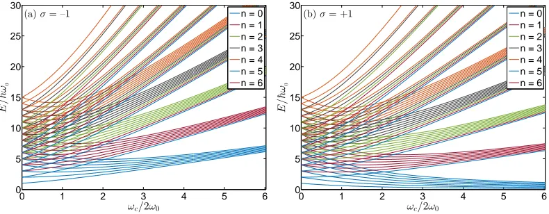
Figure 1.(a) Fock-Darwin energy spectrum withs= +1 for the first six radial numbern=0, 1, ..., 6 and for each of them the azimuthal quantum number taking the values betweenm=−6,−5, ..., 5, 6. (b) Fock-Darwin energy spectrum withs=−1 for the first six radial numbern=0, 1, ..., 6 and for each of them the azimuthal quantum number taking the values betweenm =−6,−5, ..., 5, 6. We clearly observe the confinement of the energy levels at high magnetic fields(ωc/2ω0>>1).
To obtain a more precise calculation, especially when we consider the case of strong magnetic 63
fields for the electron trapped in a quantum dot, we also take into account the electron spin of value ¯hˆσ
2 64
and magnetic momentµB, where ˆσis the Pauli spin operator andµB= 2me¯h∗. Here the spin can have
65
two possible orientations, one is↑or↓with respect to the applied external magnetic fieldBin the 66
direction of the z-axis. Therefore, we need to add the Zeeman term in the Fock-Darwin energy levels 67
Equation (4). Consequently, the new energy spectrum is given by 68
En,m,σ =h¯Ω(2n+|m|+1) +m ¯ hωc
2 −µBσB. (6)
The energy spectrum of Equation (6) is presented in Figure (1) forσ = −1 andσ = 1. It is 69
interesting to note that for high magnetic fields(ωc/2ω0>>1)things simplify in Eq. (6) and we get 70
the following expression: 71
En,m,σ = ¯ hωc
2 (n+1/2+|m|+m)−µBσB, (7)
where we observe that|m|+m=0 form<0, therefore each Landau level labelled bynhas infinite 72
degeneracy. 73
74
In our calculations along the work, we will consider a low-frequency coupling for the parabolic 75
trap given by ω0 ∼ 0.2637 THz which in terms of energy units corresponds to a coupling of 76
approximately 1.5 meV. The selection of this particular value is to compare the intensity of the 77
trap with the typical energy of intra-band optical transitions of the quantum dots [39]. The order of 78
this transition is approximately around∼1meVfor cylindrical GaAs quantum dots with effective 79
mass given bym∗∼0.067me[39,40]. 80
Throughout the discussion of this work, for the classical approach, we use the Refs. [41,42,44,45] 81
and in particular, classical thermodynamics quantities for the Fock Darwin model with spin can be 82
obtained analytically using the treatment of Kumaret. al.[46] using the partition function, which can 83
be written as: 84
ZdS = 1 2csch ¯ hβω+ 2 csch ¯ hβω− 2 cosh ¯ hβωB 2 . (8)
ω±=Ω±ωc
2 . (9)
Therefore, entropy(S(T,B)), internal energy(U(T,B))and magnetizationM(T,B)are simply given by
S(T,B) =kBlnZdS+kBT
∂lnZdS ∂T
B
, (10)
U(T,B) =kBT2
∂lnZdS ∂T
B
, (11)
M(T,B) =kBT
∂lnZdS ∂B
. (12)
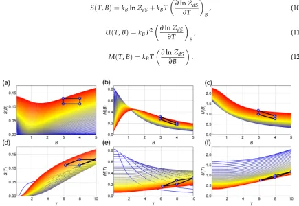
Figure 2.Classical thermodynamics quantities entropy(S), internal energy(U)and magnetization (M)as a function of temperature (T) (panels (a) to (c)) and external magnetic field (B) (panels (d) to (f)). For (a) to (c) panels the color blue to red represent temperatures from 0.1 K to 10 K respectively . For (d) to (f) panels the colors blue to red represent lower to higher external magnetic field, from 0.1 T to 5 T. The value of the parabolic trap correspond approximately to 1.5meV. Additionally, we plot the proposal cycle on each of the aforementioned thermodynamic quantities.
The Equations (10), (11) and (12) are presented in the Figure2for a parabolic trap corresponding 86
to an energy of 1.5meVtogether with the scheme of the proposed cycle. A very interesting behaviour 87
is observed for the entropy as a function of the magnetic field in the panel (a) of Figure2. For external 88
magnetic fields≤1 T, the entropy shows a decreasing behaviour as the external field increase, but for 89
values higher than 1 T contrary behaviour is found. This can be explained due to strong degeneracy 90
of the energy levels for higher magnetic fields. This degeneracy in the energy levels explains the 91
entropy growth together with the external magnetic field applied to the sample. Also, the change in 92
the behaviour of the entropy is affected by temperature, finding that the change of slope as a function 93
of external magnetic field moves away from the 1 T value to higher values in as we increase the 94
temperature of the working substance. This can be appreciated in the (a) panel of Figure (2). At the 95
same time, the magnetization shows a crossing in its behaviour as a function of magnetic field as we 96
can see in the (b) panel of Figure (2), where previous to this crossing at lower temperatures higher 97
values of magnetization are obtained. This fact will become essential for the total work extracted. 98
In the cycle that we propose, the work is directly related to the change in the magnetization of the 99
system as a function of magnetic field and temperature. On the other hand, we can observe that the 100
increases for all temperatures displayed. The reason for this is that the internal energy only depends 102
on the derivative of lnZdS(see Equation (11)) with respect to temperature while the entropy has an 103
additional term proportional to lnZdS(see Equation (10)) and the magnetization on its derivative with 104
respect to the external field (see Equation (12)). 105
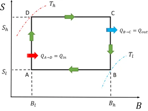
It is important to mention that the cycle operation in the counter-clockwise form starting in the A 106
point described in Figure2gives negative work extracted, so to define a thermal machine correctly, 107
we start the cycle in the point B, and we go through it in a clockwise direction. This is due to the 108
particular behaviour of the entropy as a function of magnetic field and temperature in the chosen zone 109
marked with A, B, C and D. Therefore, the cycle that will describe in the next subsection is the form of 110
B→A→D→C→B and is presented in the Figure3. 111
3. First Law of Thermodynamics and the Quantum and Classical Otto Cycle 112
Figure 3.The magnetic Otto engine represented as an entropy(S)versus a magnetic field(B)diagram. The way to perform the cycle is in the form B→A→D→C→B.
The first law of thermodynamics in a quantum context has been discussed extensively in the 113
literature. We will follow the treatment of Refs. [41,42,44], which identifies the heat transferred and 114
work performed during a thermodynamic process by means of the variation of the internal energy of 115
the system. 116
First, consider a system described by a Hamiltonian, ˆH, with discrete energy levels, En,m,σ.
117
The internal energy of the system is simply the expectation value of the Hamiltonian E = hHiˆ =
118
∑n∑m∑σpn,m,σEn,m,σ, wherepn,m,σare the corresponding occupation probabilities. The infinitesimal
119
change of the internal energy can be written as 120
dE=
∑
n
∑
m∑
σ(En,m,σdPn,m,σ+Pn,m,σdEn,m,σ), (13)
where we can identify the infinitesimal work and heat as 121
dQ:=
∑
n
∑
m∑
σEn,m,σdpn,m,σ , dW:=
∑
n
∑
m∑
σpn,m,σdEn,m,σ. (14)
Equation (13) is the formulation of the first law of thermodynamics for quantum working 122
substances. Therefore, work is then related to a change in the eigenenergies En,m,σ, which is in
123
The quantum Otto cycle is composed by four strokes: two quantum isochoric processes and two 125
quantum adiabatic processes. This cycle can be seen in Figure3replacing the value ofSlandShfor 126
Pn,m,σ(Tl,Bh)andPn,m,σ(Th,Bl)in the vertical axe respectively. For the cases that we will consider, the 127
quantum Otto cycle proceeds as follows. 128
1. Step B → A: Quantum adiabatic compression process. The systems is isolated from the 129
cold reservoir and the magnetic field is changed fromBhtoBl, withBh > Bl. During this stage the 130
populations remain constant, soPn,m,σ(Tl,Bh) =Pn,m,A σ. We recall thatP
A
n,m,σis not a thermal state. No
131
heat is exchanged during this process. 132
2. Step A→D: The systems, at constant magnetic fieldBl, is brought into contact with a hot 133
thermal reservoir at temperatureThuntil it reaches thermal equilibrium. The corresponding thermal 134
populationsPn,m,σ(Th,Bl)are given by the Boltzmann distribution with temperatureTh. No work is 135
done during this stage. 136
The heat absorbed for the working substance is given by 137
Qin=
∑
n
∑
m∑
σZ D
A En,m,σdPn,m,σ=
∑
n∑
m∑
σ E l n,m,σh
Pn,m,σ(Th,Bl)−Pn,m,A σ i
, (15)
whereEn,m,l σ is the nth eigenenergy of the system in the quantum isochoric heating process to an 138
external magnetic field of valueBl. 139
3. Step D → C: Quantum adiabatic expansion process. The system is isolated from the hot 140
reservoir, and the intensity of magnetic field is changed back fromBl toBh. During this stage the 141
populations remains constant, soPn,m,σ(Th,Bl) =Pn,m,C σ. Again, we recall thatPn,m,C σis not a thermal
142
state. No heat is exchanged during this process. 143
4. Step C→B : Quantum isochoric cooling process. The working substance atBhis brought into 144
contact with a cold thermal reservoir at temperatureTl. Therefore, the heat released is given by 145
Qout=
∑
n
∑
m∑
σZ B
C En,m,σdPn,m,σ =
∑
n∑
m∑
σ E h n,m,σh
Pn,m,σ(Tl,Bh)−Pn,m,C σ i
, (16)
whereEn,m,h σ is the nth eigenenergy of the system in the quantum isochoric heating process to an 146
external magnetic field of valueBh. 147
The net work done in a single cycle can be obtained fromW =Qin+Qout, 148
W=
∑
n
∑
m∑
σ
En,m,l σ−E
h n,m,σ
(Pn,m,σ(Th,Bl)−Pn,m,σ(Tl,Bh)), (17)
where we have used the condition of constant populations along the quantum adiabatic strokes. 149
Furthermore, the efficiency is given by 150
η= W
Qin . (18)
The main differences between the classical and quantum Otto cycle is related to the pointAand 151
Din the cycle. In classical engine, the works presented in Equation (15) and Equation (16), can be 152
calculated replacingPn,m,A σbyP(TA,Bl)andP
C
n,m,σbyP(TC,Bh)obtaining a difference between the
153
classical internal energy derived from the partition function in the form 154
Qin=U(Th,Bl)−U(TA,Bl); Qout=U(Tl,Bh)−U(TC,Bh), (19) whereTAandTCthey are determined by the condition imposed by the classical isentropic strokes. 155
If we have the classical entropy, the intermediate temperaturesTAandTCcan be determined in two 156
• Finding the relation between the magnetic field and the temperature along an isentropic trajectory 158
by solving the differential equation of first order given by 159
dS(B,T) =
∂S
∂B
T dB+
∂S
∂T
B
dT =0, (20)
which can be written as
dB dT =−
CB T∂S ∂B
T
, (21)
whereCBis the specific heat at constant magnetic field. 160
• The other possibility is to connect the entropy values of two isentropic trajectories in the form 161
S(Tl,Bh) =S(TA,Bl) S(Th,Bl) =S(TC,Bh),
(22)
finding the magnetic field in terms of the temperature, throughout numerical calculation. 162
Therefore, from the Equation (19) andW=Qin+Qout, the classical work is given by the difference 163
of four internal energy in the form 164
W =UD(Th,Bl)−UA(TA,Bl) +UB(Tl,Bh)−UC(TC,Bh), (23) In the following section, the units of temperature correspond to Kelvin (K), and the external field 165
is in units of Tesla (T). The thermodynamics quantities entropy(S), magnetization (M) and internal 166
energy(U), are in units of meVK , meVT andmeVrespectively. The total work extracted is in the units of 167
meV. The maximum values considered in our calculations for the temperatures and external magnetic 168
field are 10 K and 5 T. Therefore, for the quantum cycle calculation (i. e. Equation (17)), we use the 169
quantum numbersn = 0 ton = 10 andm = −33 tom =33 of Equation (6). The selection of this 170
particular energy levels in this model is justified for the values of the thermal populations for the hot 171
and cold temperatures of the reservoirs that we have selected. Our numerical calculations indicated 172
that the contributions of the other levels of energy can be neglected. 173
Finally, it is useful to express our results of total work extracted and efficiency in terms of the 174
relation between the highest value (Bh) and the lowest value (Bl) of the external magnetic field over 175
the sample. To do that, we use the definition of "magnetic length" which is given by 176
lB=
r
¯ h
eB, (24)
allowing us to define the parameter 177
r= lBl
lBh
= s
Bh
Bl, (25)
which represents the analogy of the compression ratio for the classical case. It is important to remember 178
that the Landau radius is inversely proportional to the magnitude of the magnetic field. Therefore, for 179
4. Results and Discussions 181
4.1. Classical Magnetic Otto Cycle 182
.
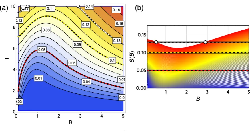
Figure 4. Solution of classical isentropic path. The panel (a) shows the entropy as a function of magnetic field (horizontal axis) and temperature (vertical axis). The level curves (constant entropy values) highlights three different values for low (red-black curve,S =0.05), middle (yellow-black curve,S=0.10) and high (white-black curve,S=0.13). The (b) panel shows the three constant values for the entropy (S=0.05,S=0.10,S=0.13) in a graphic of entropy as a function ofBfor temperatures from 1 K (blue) up to 10 K (red). Due to the form of the entropy obtained for this system, the solution forS=0.13 needs to work with temperatures higher than 10 K for an external magnetic field lower than 3 T (white dots in the (a) and (b) panel of this figure). The value of the parabolic trap corresponds to 1.5meV
The condition gives by Equation (21) (or Equation (22)) for the classical cycle give us the 183
information about the behaviour of the external magnetic field and the temperature in the adiabatic 184
stroke. In the (a) panel of Figure4, we can appreciate the level curves of the entropy functionS(T,B)
185
and in the (b) panel some examples of isentropic strokes in a plot ofS(B)vsBfor different temperatures. 186
That example shows three cases of constant entropy for a low (red-black curve,S = 0.05), middle 187
(yellow-black curve,S =0.10) and high (white-black curve,S =0.13). We observe in the (a) panel 188
of Figure (4) that there is a zone where the external field grows with the temperature of the sample 189
and a zone where the opposite happens in order to maintain the entropy constant. At low working 190
temperatures, the behaviour changes nearB = 1 T, while as the temperature increases, the slope 191
change occurs at higher values of the magnetic field, approachingB=2 T. Secondly, if we observe 192
the (b) panel of Figure (4) the case forS=0.13 (white-black line), we have a restricted area for field 193
values lower to 3 T if we work with a maximum temperature of 10 K. Therefore, it is not arbitrary 194
the movement of the magnetic field if we think in a thermodynamic magnetic Otto cycle with two 195
temperature reservoirs fixed at some specific values, more specifically, the reservoir associated to the 196
hot temperature in the cycle. Also, the Figure4is the solution ofS(T,B) =constant, obtained from 197
the differential Equation (21) with different conditions (i. e. distinct values of the constant value ofS). 198
Therefore, panel (a) of Figure4depicts all family of solutions for the isentropic stroke of the engine of 199
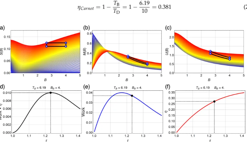
In our first example displayed in the Figure (5), the B point has the value of the external field 201
given byBh=4 T and a temperature ofTB=6.19 K. The value of the temperature for the D point is 202
fixed toTD=10 K. Therefore, the Carnot efficiency of the proposal cycle is given by 203
ηCarnot=1− TB
TD
=1−6.19
10 =0.381 (26)
Figure 5.Proposed magnetic Otto cycle showing three different thermodynamics quantities, Entropy (S), Magnetization (M) and Internal Energy (U) ((a) to (c) panel respectively) as a function of the external magnetic field and different temperatures from 0.1K(blue) to 10K(red). Panel (d) shows the total work extracted multiplied by efficiency(Wη), (e) shows the total work extracted(W)and (f) the
efficiency(η)for the classical cycle. The black points in the panels (d) to (f) represent exactly the cycle
B→A→D→C→B, presented in the panels (a) to (c). The value of the parabolic trap corresponds to 1.5meV. The fixed temperatures areTB=6.19 K andTD=10 K.
The low central panel (e) of the Figure5shows different values of total work extracted (W)
204
varying the value of BD from 4 T to 1.99 T. This variation in the external field is reflected in the 205
movement ofrin the form ofr=qB4
l. Therefore,ris in the range of 1≤r≤1.41. The parabolic trap 206
is fixed to the value of 1.5meVand the effective mass in the value ofm∗=0.067me. In particular, the 207
(a) to (c) panels of the Figure5shows the exact paths for the magnetic cycle for the maximum point 208
obtained when multiplyingW((e) panel) and the efficiency (η, (f) panel). That point corresponds to 209
r∼1.22 (black point in the (d) to (f) panels of the Figure5and constitutes the best configuration of the 210
systems in order to obtain the bestWwith the betterηthrough the cycle. Also,Wandηare presented 211
in (e) and (f) panel of Figure5for the optimal value ofrparameter mentioned before. We observe that 212
Wobtained for that point is in the order of∼0.038meVwith an efficiency ofη∼0.28. We verified the 213
numeric value of total work extracted using the area enclosed by the cycle in the graph ofMversus 214
Bof Figure5panel (b) due to the fact that the work isW=−R
MdB[37,42,44] when the parameter 215
changed during the operation of the engine is the external field. On the other hand, to obtain the 216
solid lines presented in the (d) to (f) panels in Figure5we need to make different cycles configuration 217
keeping the values of the isothermal fixed as can be appreciated in theSupplemental Material I, made 218
with the Mathematica software [43], where we show each shape that the cycle must have to generate a 219
point of work in specific. It is important to recall that we never reach the optimal value ofη=0.381, 220
i.e. the Carnot efficiency. 221
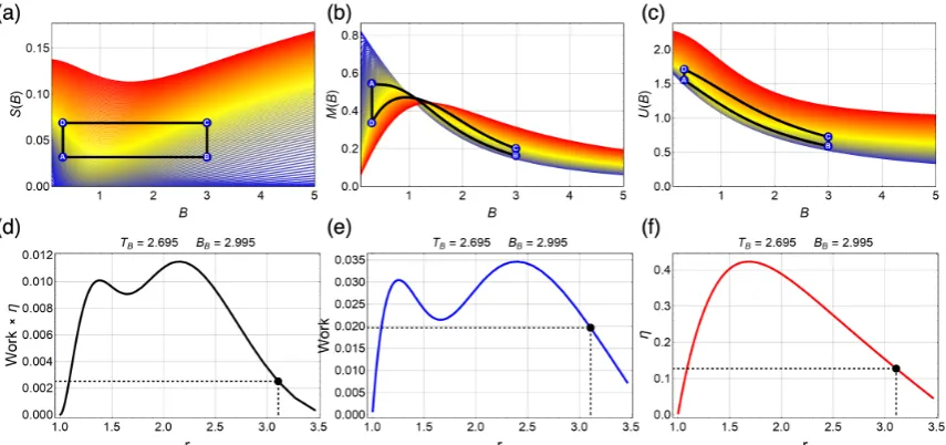
Due to the change of behaviour in the entropy as a function of the external field, we obtain a 222
point, the entropy decrease as function of the external field(B)and after that point entropy begins 224
to increase. This fact can be used to explore the magnetic cycle in that zone finding an oscillatory 225
behaviour forW. In the Figure6we show the cycle with operating temperaturesTB =2.69 K and 226
TD=5.40 K and external magnetic field moving between 2.995 T to 0.250 T and consequently, ther 227
parameter move from 1 to 3.46. First, we observe a decreasing efficiency forr>1.75 in the (f) panel of 228
Figure6with a maximum value ofη∼0.43 forr∼1.75. Therefore, for this configuration, the Carnot 229
efficiency (ηCarnot ∼0.5 for this case) also can not be reached. In order to compare this results with the 230
previously discussed ( when we avoid this particular region ) we can see from the (f) panel of Figure5
231
that the efficiency asymptotically approaches to the efficiency of Carnot if we increase the intensity of 232
the external magnetic field of the starting point of the cycle (point B). 233
Figure 6. Proposed magnetic Otto cycle in three different thermodynamics quantities, Entropy, Magnetization and internal energy ((a) to (c) panels respectively) as a function of the external magnetic field and different temperatures from 0.1K(blue) to 10K(red). Total work extracted multiplied by efficiency(Wη)(d) total work extracted(W)(e) and efficiency(η)(d) for the cycle. The black point in
the panels (d) to (f) represent the value of 0.02meVof total work extracted and corresponds exactly to the cycle B→A→D→C→B, showed in the panels (a) to (c). The value of the parabolic trap correspond to 1.5meV. The fixed temperatures areTB=2.69 K andTD=5.40 K.
From panel (b) of Figure6, we can understand the oscillations inWinterpreting these results 234
using the expressionW=−R
MdB. Observing the (a) to (c) panels of Figure6, the presented A,B,C,D 235
points correspond to the black point displayed in the (d) to (f) panels where we see that the work is 236
still greater than zero but close to a vanishing situation. The reason why there is still positive work in 237
this point under study, is that the total area enclosed to the right of the crossing point is larger than the 238
other in the left. The magnetization presented in the (b) panel of Figure6in the zone around the range 239
of external magnetic field explored for this case (from 2.995 to 0.250T) clearly reverses his behaviour 240
and presents a crossing point close toB ∼1.2 T for different temperatures. The area to the right of 241
that point can be interpreted as a positive contribution toWwhile the left area contributes to negative 242
Figure 7.Work, efficiency and work multiply by efficiency ((a) to (c) panels ) for different values ofTD forTB=2.69 fixed. The value of the parabolic trap corresponds to 1.5meV.
To explore if these oscillations inW are still obtained for higher temperature ranges, we plot 244
in Figure7the workWfor different values ofTDwithTB = 2.69 K fixed. We note that for higher 245
temperatures than 7 K the oscillations found before disappear. It is only a reinforcement that the 246
quantum effects of the working substance are only significant at low temperatures. On the other hand, 247
as we expect,Wgrows as the difference between the temperature reservoir is larger as we can see 248
from the (a) panel of Figure7. However, for this case, the efficiency obtained is increasingly lower for 249
increasingly larger temperature differences as we can appreciate from the panel (b) of Figure7. 250
4.2. Magnetic Quantum Otto Cycle 251
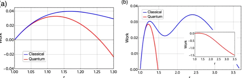
Next we show the results of the evaluation of the quantum version of this magnetic Otto cycle 252
for the same cases shown in Figure5and Figure6. In the (a) panel of Figure8, we plot the classical 253
work (blue line) and the quantum work (red line) for the same sets of parameters of Figure5. First, we 254
note that the classical and quantum work are equal up to the value ofr∼1.07. That means for close 255
values of the starting external magnetic field to the B point we do not notice a difference between the 256
classic and quantum formulation of the Otto cycle. Also, in (a) panel Figure8, we found that we have 257
a transition from positive work to negative work not reflected in the classic scenario close tor∼1.36. 258
Figure 8.(a) Total work extracted for classical (blue line) and quantum version of Otto cycle (red line). The parameters for this case displayed are :TD=10 K,TB=6.19 K andBB=4 T as starting value of the external magnetic field. The value ofBDmoves from 4 T to 1.99 T and this variation is reflected in the movement ofrin the form ofr=qB4
D, same parameter as the results shown in Figure5. (b) Total
work extracted (W) presented in the (e) panel of Figure6versus the values obtaining in the quantum version of the Otto cycle. The parameters for this figure areTD=5.40K,TB=2.69KandBB=2.995 T andBDmoves from 2.995 to 0.250 T. The parabolic trap is fixed to the value of 1.5meVand the effective mass value ofm∗ =0.067me.
Additionally, we observe that the maximum positive value of the total work extracted for the 259
quantum version of Otto cycle is reduced by approximately 0.01 meV compared to the classical 260
presented in the (e) panel of Figure6. Moreover, we found a transition from positive to negative work 262
at some value of therparameter. This is dramatically reflected in the (b) panel of Figure8, where the 263
absolute value ofWis highly increased as compared with the classical approach. 264
Figure 9.Total quantum work extracted(W)per energy level for the case ofσ=1 ((a) panel) and for
the case ofσ=−1 ((b) panel). The line marked (in the two panels) with circles correspond to the sum
of all contributions of the energy level for each spin. The parameters used for this figure are the same as the one used in panel (b) of Figure(8).
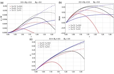
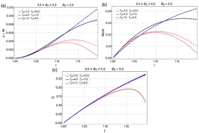
Figure 10.η×W(a), total work extracted (b) and (c) efficiency for the case of∆T=Th−Tl=3Kfor
different regions of temperature parameter for classical approach (solid line) and quantum version of the magnetic Otto cycle (dotted line). For all graphics, we use the initial external magnetic field in the value ofBB=3.5 T and the minimum value of the field,BDmoves between 3.5 T to 2.0 T. Therefore,
therparameter moves between 1≤r≤1.32. The parabolic trap is fixed to the value of 1.5meVand the effective mass value ofm∗=0.067me.
In Figure9, we present the workWper energy level and spin value for the most important values 265
of our numerical calculations. We use the same parameter as in panel (b) of Figure8. We observe that 266
the contribution given byσ=1 are positive up torclose tor∼1.6 being the energy levelsE0,−1,E0,−2 267
found that all contributions per energy level are negative. Therefore, the small region of positive work 269
found in panel (b) of Figure8can be only associated to the spin up (σ=1) contributions. 270
To explore other operation regions for the magnetic Otto cycle, we calculate the total work 271
extracted and efficiency for the same∆T =Th−Tlin a broad range of temperatures and the same 272
∆Bmax =1.5 T in different regions of the external magnetic field for the classical cycle and its quantum 273
version. This is displayed in Figure10and Figure11where the dotted lines represent the classical 274
results and the solid lines the quantum results. The three regions of temperature selected for this two 275
figures are between 1 K to 4 K (blue lines), 4 K to 7 K (black lines) and 7 K to 10 K (red lines). First, 276
we treat the case ofBB = 3.5 T andBDmoving from 3.5 T to 2.0 T in the Figure10, where we note 277
large differences between the classical and quantum results forWas can be seen in the (b) panel of 278
that figure. On the other hand, if we observe the region of 3.5≤BD≤5.0 T for aBBfixed shown in 279
the (b) panel of Figure11, the work and efficiency for the region of 1 K to 4 K and 4 K to 7 K presents 280
similar behaviour for the classical and quantum version. Only the case of 7 K to 10 K shows a larger 281
difference between this two approaches. For the case of the efficiency, we note in the (c) panel of Figure 282
10a major difference between the classical results and quantum results compare with the presented in 283
(c) panel of Figure11and this is consistent with the reported results for the workW. 284
Figure 11.η×W(a), total work extracted (b) and (c) efficiency for the case of∆T=Th−Tl=3Kfor
different regions of temperature parameter. For all cases, we use the initial external magnetic field at the value ofBB=5.0 T and the minimum value of the field,BDmoves between 5.0 T to 3.5 T. Therefore,
therparameter moves between 1≤r≤1.19. The parabolic trap is fixed to the value of 1.5meVand the effective mass value ofm∗=0.067me.
5. Conclusions 285
In this work, we explored the classical and quantum magnetic Otto cycle for an ensemble 286
of non-interacting electrons with intrinsic spin where each one is trapped inside a semiconductor 287
quantum dot modeled by a parabolic potential. We analyzed all relevant thermodynamics quantities, 288
we found in particular for the entropy as a function of the external magnetic field, a zone where it 289
diminishes as the field increases but then it increases again at larger fields, at all temperatures. This is a 290
consequence of the infinite degeneracy that the system has at high magnetic fields, thus increasing its 291
on the work area in temperatures and magnetic fields. We find oscillations in the total work extracted 293
near the zone of slope change in the behaviour of entropy when the cycle is classically evaluated. 294
Additionally, we evaluate the total work and efficiency for classical and quantum Otto cycle, always 295
finding, in the explored zones, that the work and efficiency for the classical cycle are larger than their 296
quantum counterpart. 297
298
Acknowledgments:F. J. P. acknowledges the financial support of FONDECYT-postdoctoral 3170010, and D. Z. 299
acknowledges to USM-DGIIP. P. Vargas acknowledge support from Financiamiento Basal para Centros Científicos 300
y Tecnológicos de Excelencia, under Project No. FB 0807 (Chile), authors acknowledge to DTI-USM for the use of 301
"Mathematica Online Unlimited Site" at the Universidad Técnica Federico Santa María 302
Author Contributions:F. J. P. , G. A. and P. V. conceived the idea and formulated the theory. O. N., D. Z and A .G. 303
built the computer program and edited figures. A. S. N. and P. A. O. contributed to discussions during the entire 304
work and the corresponding editing of the same. F. J. P. wrote the paper. All authors have read and approved the 305
final manuscript. 306
Conflicts of Interest:The authors declare no conflict of interest. 307
References 308
1. Scovil, H.E.D.; Schulz-DuBois, D.O. Three-Level masers as a heat engines.Phys. Rev. Lett.1959,2, 262-263. 309
2. Feldmann, T.; Geva, E.; Kosloff, R. and Salamon, P. Heat engines in finite time governed by master equations. 310
American Journal of Physics1996,64, 485. 311
3. Feldmann, T. and Kosloff, R. Characteristics of the limit cycle of a reciprocating quantum heat engine.Phys.
312
Rev. E2004,70, 046110. 313
4. Rezek, Y. and Kosloff, R. Irreversible performance of a quantum harmonic heat engine.New Journal of Physics
314
2006,8, 83. 315
5. Henrich, M. J.; Rempp, F. and Mahler, G. Quantum thermodynamic Otto machines: A spin-system approach. 316
The European Physical Journal Special Topics2007,151, 157. 317
6. Quan, H. T.; Liu, Y. -x.; Sun, C. P., and Nori, F. Quantum thermodynamic cycles and quantum heat engines. 318
Phys. Rev. E2007,76, 031105. 031105 (2007). 319
7. He, J.; He, X. and Tang, W. The performance characteristics of an irreversible quantum Otto harmonic 320
refrigeration cycle.Science in China Series G: Physics, Mechanics and Astronomy2009,52, 1317. 321
8. Liu, S.; Ou, C. Maximum Power Output of Quantum Heat Engine with Energy Bath.Entropy2016,18, 205. 322
9. Scully, M.O.; Zubairy, M.S.; Agarwal, G.S.; Walther, H. Extracting work from a single heath bath via vanishing 323
quantum coherence.Science2003,299, 862–864. 324
10. Scully, M.O.; Zubairy, M.S.; Dorfmann, K.E.; Kim, M.B.; Svidzinsky, A. Quantum heat engine power can be 325
increased by noise-induced coherence.Proc. Natl. Acad. Sci. USA2011,108, 15097–15100. 326
11. Bender, C.M.; Brody, D.C.; Meister, B.K. Quantum mechanical Carnot engine.J. Phys. A Math. Gen.2000, 327
33, 4427. 328
12. Bender, C.M.; Brody, D.C.; Meister, B.K. Entropy and temperature of quantum Carnot engine.Proc. R. Soc.
329
Lond. A2002,458, 1519. 330
13. Wang, J.H.; Wu, Z.Q.; He, J. Quantum Otto engine of a two-level atom with single-mode fields.Phys. Rev. E
331
2012,85, 041148. 332
14. Huang, X.L.; Xu, H.; Niu, X.Y.; Fu, Y.D. A special entangled quantum heat engine based on the two-qubit 333
Heisenberg XX model.Phys. Scr.2013,88, 065008. 334
15. Muñoz, E.; Peña, F.J. Quantum heat engine in the relativistic limit: The case of Dirac particle.Phys. Rev. E
335
2012,86, 061108. 336
16. Quan, H.T. Quantum thermodynamic cycles and quantum heat engines (II).Phys. Rev. E2009,79, 041129. 337
17. Zheng, Y.; Polleti, D. Work and efficiency of quantum Otto cycles in power-law trapping potentials. 338
Phys. Rev. E2014,90, 012145. 339
18. Cui, Y.Y.; Chem, X.; Muga, J.G. Transient Particle Energies in Shortcuts to Adiabatic Expansions of Harmonic 340
Traps.J. Phys. Chem. A2016,120, 2962. 341
19. Beau, M.; Jaramillo, J.; del Campo, A. Scaling-up Quantum Heat Engines Efficiently via Shortcuts to 342
20. Deng, J.; Wang, Q.; Liu, Z.; Hänggi, P.; Gong, J. Boosting work characteristics and overall heat-engine 344
performance via shortcuts to adibaticity: Quantum and classical systems.Phys. Rev. E2013,88, 062122. 345
21. Wang, J.; He, J.; He, X. Performance analysis of a two-state quantum heat engine working with a single-mode 346
radiation field in a cavity.Phys. Rev. E2011,84, 041127. 347
22. Abe, S. Maximum-power quantum-mechanical Carnot engine.Phys. Rev. E2011,83, 041117. 348
23. Wang, J.H.; He, J.Z. Optimization on a three-level heat engine working with two noninteracting fermions in 349
a one-dimensional box trap.J. App. Phys.2012,111, 043505. 350
24. Wang, R.; Wang, J.; He, J.; Ma, Y. Performance of a multilevel quantum heat engine of an ideal N-particle 351
Fermi system.Phys. Rev. E2012,86, 021133. 352
25. Jaramillo, J.; Beau, M.; del Campo, A. Quantum supremacy of many-particle thermal machines.New J. Phys.
353
2016,18, 075019. 354
26. del Campo, A.; Goold, J.; Paternostro, M. More bang for your buck: Super-adiabatic quantum engines. 355
Sci. Rep. 42017, 14391. 356
27. Huang, X.L.; Niu, X.Y.; Xiu, X.M.; Yi, X.X. Quantum Stirling heat engine and refrigerator with single and 357
coupled spin systems.Eur. Phys. J. D2014,68, 32. 358
28. Su, S.H.; Luo, X.Q.; Chen, J.C.; Sun, C.P. Angle-dependent quantum Otto heat engine based on coherent 359
dipole-dipole coupling.EPL2016,115, 30002. 360
29. Kosloff, R.; Rezek, Y. The Quantum Harmonic Otto Cycle.Entropy2017,19, 136. 361
30. Roßnagel, J.; Dawkins, T.K.; Tolazzi, N.K.; Abah, O.; Lutz, E.; Kaler-Schmidt, F.; Singer, K. A single-atom 362
heat engine.Science2016,352, 325. 363
31. Dong, C.D.; Lefkidis, G.; Hübner, W. Quantum Isobaric Process inNi2.J. Supercond. Nov. Magn.2013,26, 364
1589–1594. 365
32. Dong, C.D.; Lefkidis, G.; Hübner, W. Magnetic quantum diesel inNi2.Phys. Rev. B2013,88, 214421. 366
33. Hübner, W.; Lefkidis, G; Dong, C.D.; Chaudhuri, D. Spin-dependent Otto quantum heat engine based on a 367
molecular substance.Phys. Rev. B2014,90, 024401. 368
34. Mehta, V.; Johal, R.S. Quantum Otto engine with exchange coupling in the presence of level degeneracy. 369
Phys. Rev. E 2017,96, 032110. 370
35. Azimi, M.; Chorotorlisvili, L.; Mishra, S.K.; Vekua, T.; Hübner, W.; Berakdar, J. Quantum Otto heat engine 371
based on a multiferroic chain working substance.New J. Phys.2014,16, 063018. 372
36. Chotorlishvili, L.; Azimi, M.; Stagraczy ´nski, S.; Toklikishvili, Z.; Schüler, M.; Berakdar, J. Superadiabatic 373
quantum heat engine with a multiferroic working medium.Phys. Rev. E2016,94, 032116. 374
37. Muñoz, E.; Peña, F.J. Magnetically driven quantum heat engine.Phys. Rev. E2014,89, 052107. 375
38. Mani, R.G.; Smet, J.H.; von Klitzing, K.; Narayanamurti, V.; Johnson, W.B.; Umansky, V. Zero-resistance 376
states induced by electromagnetic-wave excitation in GaAs/AlGaAs heterostructures. Nature2002, 420, 377
646–650. 378
39. Jacak, L.; Hawrylak, P. and Wójs,Quantum Dots, Springer-Verlag, 1998. 379
40. Muñoz, E.; Barticevic, Z. and Pacheco, M. Electronic spectrum of a two-dimensional quantum dot array in 380
the presence of electric and magnetic fields in the Hall configuration.Phys. Rev. B200571, 165301. 381
41. Quan, H.T.; Zhang, P.; Sun, C.P. Quantum heat engine with multilevel quantum systems.Phys. Rev. E2005, 382
72, 056110. 383
42. Peña, F.J.; Muñoz, E. Magnetostrain-driven quantum heat engine on a graphene flake.Phys. Rev. E2015, 384
91, 052152. 385
43. Wolfram Research, Inc., Mathematica, Version 11.3, Champaign, IL (2018). 386
44. Muñoz, E.; Peña, F.J.; González, A. Magnetically-Driven Quantum Heat Engines: The Quasi-Static Limit of 387
Their Efficiency.Entropy2016,18, 173. 388
45. Callen, H. B.Thermodynamics and an introduction to thermostatistics, John Wiley & sons 1985. 389
46. Kumar, J.; Sreeram P. A. and Dattagupta, S., Low-temperature thermodynamics in the context of dissipative 390