Comparing Markov Chain Samplers for Molecular Simulation

Article

Comparing Markov Chain Samplers for Molecular

Simulation

Robert D Skeel1,† ID _{and Youhan Fang}2ID

1 _{Purdue University; [email protected]} 2 _{Purdue University; [email protected]}

* Correspondence: [email protected] † Current address: Arizona State University

Abstract: Markov chain Monte Carlo sampling propagators, including numerical integrators for

1

stochastic dynamics, are central to the calculation of thermodynamic quantities and determination of

2

structure for molecular systems. Efficiency is paramount, and to a great extent, this is determined by the

3

integrated autocorrelation time (IAcT). This quantity varies depending on the observable that is being

4

estimated. It is suggested that it is the maximum of the IAcT over all observables that is the relevant

5

metric. Reviewed here is a method for estimating this quantity. For reversible propagators (which are

6

those that satisfy detailed balance), the maximum IAcT is determined by the spectral gap in the forward

7

transfer operator, but for irreversible propagators, the maximum IAcT can be far less than or greater

8

than what might be inferred from the spectral gap. This is consistent with recent theoretical results

9

(not to mention past practical experience) suggesting that irreversible propagators generally perform

10

better if not much better than reversible ones. Typical irreversible propagators involve a parameter

11

controlling the mix of ballistic and diffusive movement. To gain insight into the effect of the damping

12

parameter for Langevin dynamics, its optimal value is obtained here for a multidimensional quadratic

13

potential energy function.

14

Keywords:Markov chain Monte Carlo; stochastic dynamics integrators; decorrelation time; integrated

15

autocorrelation time.

16

1. Summary 17

Thermodynamic and structural properties of a molecular system can be precisely defined as

18

expectations of ensemble-dependent functions of its configurations. The calculation of such expectations

19

is feasible only with the use of Markov chain Monte Carlo (MCMC) methods or approximations thereof.

20

Considered here are sampling propagators that do not compromise the Markov property. Included are

21

unbiased samplers that conditionally accept proposed moves and biased samplers that unconditionally

22

accept such moves, in particular, discretized stochastic dynamics. Many such sampling propagators

23

are proposed in the literature, and, in virtually all cases, experiments are conducted to substantiate

24

claims of superiority. Too often though, a good metric is not used to measure the computational cost of a

25

propagator. The aim of this article is threefold: First, to explore some practicalities related to measuring

26

the efficiency of a propagator. Second, to highlight the superior efficiency of irreversible propagators,

27

namely, those that do not satisfy detailed balance. Third, to provide some insight into the optimal mix of

28

diffusive and ballistic movement for Langevin dynamics.

29

LetρQ(q), q = [q1,q2, . . . ,qν]T, denote the probability density function corresponding to the 30

ensemble of interest. This function is assumed to be known only up to a multiplicative factor. An

31

observable is an expectationE[u(Q)] =R u(q)ρQ(q)dqfor some “preobservable”u(q). This can be 32

estimated by the mean ¯UN = (1/N)∑nN=−01u(Qn), where the random valuesQnare obtained from a 33

Markov chainQ0→Q1→ · · · →QN−1that samples fromρQ(q). Note the use here of upper case to 34

denote random variables.

35

In practice, sampling performance is improved if the configuration variablesqare augmented with auxiliary variablesp, e.g., momenta, yielding phase space variablesz= (q,p). The probablity density is extended toρ(q,p)so that

Z

ρ(q,p)dp=ρQ(q),

and an MCMC scheme is constructed to produce a chainZ0→Z1→ · · · →ZN−1whereZ= (Q,P). 36

The samples from the chain tend to be highly correlated, and this greatly reduces the convergence rate asN→+∞. As explained in Sec.2, the variance of an estimate forE[u(Z)]is

Var[U¯N] =

τ

NVar[u(Z)] +O( 1

N2) (1)

whereτis theintegrated autocorrelation time(IAcT) foru(z). Theeffective sample sizeis thereforeN/τ, and

37

the appropriate metric for evaluating a propagator is the effective sample size divided by the computing

38

time.

39

In a great many practical simulations, the effective sample size is probably close to zero. One

40

can disagree on the significance of such simulations [1]. In any case, for the comparison of sampling

41

algorithms, it is possible to choose molecular systems, restrained if necessary, for which it is feasible to

42

attain a decent effective sample size.

43

Often thespectral gapis cited as the relevant quantity. To understand its role, it is helpful to express

44

ideas in a direct way as in Ref. [2]. As detailed in Sec.2, introduce a forward transfer operatorF to

45

express the ratioρn/ρin terms ofρn−1/ρ, whereρn(z)is the probablity density forZn. LetF0=F − E 46

whereEudenote thefunctionwith constant valueE[u(Z)], Assume that the operatorF0has its spectrum 47

strictly inside the unit circle, as it does in practice. The error in(1/N)∑N−1

n=0 ρn(z)can be shown [1] to be

48

“proportional to”(1− F0)−1and therefore to the reciprocal of the spectral gap|1−λ2|, whereλ2is a 49

nonunit eigenvalue ofF nearest 1.

50

Estimates of the IAcT are obtained by summing the terms of the autocorrelation function, which

51

is constructed from autocovariances of increasing time lags normalized by the (lag zero) covariance.

52

Each term contributes a roughly equal statistical error but a signal that decays as the lag time increases.

53

Therefore, in practice, the terms are weighted by a function called a lag window. The lag window must

54

be tailored to the autocorrelation function, and choosing a suitable lag window is very difficult, as

55

mentioned in Sec.2.1.

56

Reliable estimates of the IAcT are impractical in general. Sec. 3 introduces the concept of quasi-reliability, which aims to enforce a necessary condition for reliable estimates. Informally, the goal is to ensure good coverage of those “parts” of phase space that has been explored, to reduce the possibility of missing an opening to an unexplored part of phase space. More precisely, for an arbitrary subset of phase space, we ask that the proportion of samples in that subset differ from its expectation by no more than some tolerancetol, with, say, 95% confidence. This is shown to be true if the IAcTτfor any preobservableu(z)satisfiesτ≤tol2N. The maximum IAcTτmaxis the greatest eigenvalue of

G=1− E+F0(1− F0)−1+F0†(1− F0†)−1, (2)

where†denotes the adjoint with respect to the inner product

hv,ui= Z

For a reversible propagator, whereF†_=F,

τmaxis 1 less than twice the reciprocal of the spectral gap. 57

However, for an irreversible propagator, it can be much smaller, as demonstrated by a simple example in

58

Sec.4.1, or larger as in Sec.5. As a practical algorithm, it is suggested to obtain the maximum IAcT by

59

first discretizing the space of preobservables. Consideration of a quadratic energy potential suggests

60

using a linear combination of phase space variables (and possibly quadratic terms in these variables).

61

The idea of seeking the preobservable that maximizes the IAcT is suggested already in Ref. [3],

62

which considers a set of indicator functions as preobservables and uses the greatest IAcT of these to

63

assess sampling thoroughness. In general, maximizing over a linear combination of preobservables

64

can lead to a much larger result than taking the maximum of them individually, due to correlations

65

that might exist between different preobservables. This does not necessarily apply, however, to those

66

considered in Refs. [1,3].

67

Sec.3.1notes that that typical irreversible propagators, termed “quasi-reversible” here, have a

68

forward transfer operator F = RF¯ where each of ¯F and R is reversible and R2 _{= 1. For such} 69

propagators, the estimation ofτmaxsimplifies somewhat. 70

Theoretical results [4] indicate that adding irreversibility reduces the autocorrelation times of

71

observables. Sec.4gives a couple of very elementary examples illustrating the dramatic increase inτmax 72

if an irreversible propagatorFis replaced by its reversible “counterpart” 1₂(F+F†_). 73

Discretized Langevin dynamics is a particularly effective general-purpose propagator.

74

Unfortunately, one must specify a value for the damping coefficientγ. Sec.5analyzesτmaxfor a quadratic 75

potential and obtains an optimal value for the coefficient, namely, the value(3/8)1/2=0.612· · · times

76

the critical damping coefficent for lowest frequencyω1. This value is such that the lowest frequency 77

mode is moderately underdamped, with higher frequencies increasingly underdamped.

78

2. Preliminaries 79

Assuming thatZ0has probability densityρ(z), the variance of the estimateUNis exactly

Var[UN] =

1

NVar[u(Z)] 1+2

N−1

∑

k=1

1− k

N _C(k)

C(0) !

where the autocovariances

C(k) =_E[(u(Z0)−E[u(Z0)]) (u(Zk)−E[u(Zk)])].

The limitN→+∞gives Eq, (1) where the integrated autocorrelation time

τ=1+2

+∞

∑

k=1 C(k)

C(0). (3)

As an example of augmenting configuration space, considerρ(q,p)∝exp(−β(V(q)) +1₂pTM−1p)) where p = [p1,p2, . . . ,pν]T. A good propagator for this is the BAOAB integrator [5] for Langevin

dynamics, whose equations are

dQt=M−1Ptdt, dPt=F(Qt)dt−γPtdt+

s 2γ

β M1/2dWt, (4) where M is a matrix chosen to compress the range of vibrational frequencies, F(q) = −∇V(q),

80

M1/2MT1/2 = M, andWt is a vector of independent standard Wiener processes. Each step of the 81

integrator consists of the following substeps:

82

B: P0n =Pn−1+12∆tF(Qn−1), 83

A: Q0n =Qn−1+12∆tM−1P0n,

O: P00n =exp(−γ∆t)P0n+

p

1−exp(−2γ∆t)β−1/2M1/2Rn,

85

A: Qn =Q0n+12∆tM

−1_P00

n,

86

B: Pn =P00n+12∆tF(Qn), 87

whereRnis a vector of independent standard Gaussian random variables. The samples generated from

88

this process are shown [6] to be those from a distribution that differs from the correct one by onlyO(∆t2).

89

The special choiceγ=1/(2∆t)is the Euler-Leimkuhler-Matthews integrator [5] for Brownian dynamics

90

with step sizeδt=∆t2/2. Remarkably, the invariant density of this integrator differs from the correct

91

one by onlyO(δt2). This integrator can be expressed as a Markov chainQ₁0 →Q0₂→ · · · →Q0_N−1in

92

configuration space, with propagator

93

Qn =Q0n+12

√

2δtβ−1/2_M−T 1/2Rn, 94

Q0_n+1=Qn+δtM−1F(Qn) +1₂

√

2δtβ−1/2M_1/2−TRn,

95

which is a discretization of Brownian dynamics

dQt=M−1F(Qt)dt+

s 2 βM

−T

1/2dWt. (5)

The desired samples{Qn}are available as part of the process (and, as a theoretical observation, they

96

can be recovered from the Markov chain{Q0_n}alone, by eliminatingRnin the two equations above and

97

solving forQn).

98

For any MCMC propagator, the forward transfer operator is defined so that

un=Fun−1

whereun(z) =ρn(z)/ρ(z)andρn(z)is the probability density forZn. In particular,

Fun−1(z) = 1 ρ(z)

Z

ρ(z|z0)un−1(z0)ρ(z0)dz0

whereρ(z|z0)is the transition probablity for the chain. The operatorF has an eigenfunctionϕ1(z)≡1 99

for eigenvalueλ1=1. 100

A reversible propagator is one that satisfies detailed balance, which means that

ρ(z0|z)ρ(z) =ρ(z|z0)ρ(z0).

Detailed balance is equivalent to F† _{= F, where the adjoint F}† _{is defined by the condition that} 101

hFv,ui=hv,F†_{uifor arbitraryu(z)andv(z). The BAOAB integrator is not reversible as a sampling} 102

propagator, except for the special caseγ=1/(2∆t); but a scheme consisting of a fixed number of BAOAB

103

steps followed by a momenta flip is reversible. The unmodified BAOAB integrator is, however, in a class

104

of “quasi-reversible” integrators introduced in Sec.3.1.

105

As a model problem for Brownian dynamics, given by Eq. (5), considerF(q) =−mω2q. Changing variablesQt= (mβ)−1/2Q0tand dropping the prime gives the simple stochastic differential equation

dQt=−ω2Qtdt+

√

2 dWt, (6)

whereW(t)denotes a standard Wiener process. A perfect realization ofQ(t)at discrete points is obtained by the reversible propagator

Qn =exp(−ω2δt)Qn−1+ q

1−exp(−2ω2δt)1

The probablity densityρ(q,t)forQ(t)satisfies the Fokker-Planck equation(∂/∂t)ρ= (∂/∂a)(ω2qρ) + (∂2_/∂q2_{)ρ. Writing ρ(q,t) = u(q,t)ρ(q) gives (∂/∂t)u = −ω}2_{q(∂/∂q)u+ (∂}2_/∂q2_{)u. The operator} on the right-hand side has eigenfunctions u(q) = Hek(ωq) with eigenvalues −kω2 for k =

0, 1, . . .. The modified version of the Hermite polynomial of degree k is given by Hek(x) =

(−1)kexp(x2/2)(dn/dxn)exp(−x2/2). The forward transfer operator F for the propagator defined by Eq. (7) has these same eigenfunctions and has eigenvaluesλk+1 = exp(−kω2δt)for k = 1, 2, . . .. The spectral gap is 1−exp(−ω2δt). In the multidimensional case with normal mode frequencies 0 < ω1 ≤ ω2 ≤ · · · ≤ ων, the time step δt is some fraction, say 12, of 1/ων2 and the spectral

gap is very nearly 1₂ω2₁/ω2_ν. To see the applicability to practical numerical integrators, consider the Euler-Leimkuhler-Matthews discretization of Eq. (6):

Q0n= (1−ω2δt)Q0n−1+ (1− 1 2ω

2_δt)√₂ ω2δt1

ωRn. (8)

Comparing Eqs. (8) and (7) and equating the coefficients of the two terms on their right-hand sides

106

enables Eq. (8) to be written in the form of Eq. (7) with modified values forωandδt. In particular,

107

the modified value of exp(−ω2δt)is 1−ω2δt, so spectral gap is exactlyω2δt. In the multidimensional

108

case, whereω2₁δt1, the spectral gap for the discrete stochastics isvery nearlythat of the continuous

109

stochastics.

110

2.1. Estimating integrated autocorrelation time

111

Suggested [7] as a covariance estimate is the quantity

CN(k) = 1

N

N−k−1

∑

n=0

(u(zn)−UN)(u(zn+k)−UN),

with justification in Ref. [8, pp. 323–324].

112

The use of all possible termsCN(k)/CN(0)in Eq. (3) to estimate the IAcT does not converge in the

limitN →+∞, so, in practice, alag window w(k)is used to increasingly damp terms as the noise to signal ratio increases:

τ≈1+

N−1

∑

k=1

w(k)CN(k) CN(0).

An interesting algorithm calledacorfor estimating the IAcT is available on the web [9]. Estimating

113

the IAcT can be quite difficult, andacorcan give unsatisfactory results. An attempt to improve it [1] is

114

at best marginally successful. For reversible methods, there are properties of the autocorrelation function

115

that may be useful for improving estimates of it [7].

116

3. Quasi-reliable Estimates of Sampling Thoroughness 117

The idea of quasi-reliability is to require that the sample sizeNbe large enough that, with say 95% confidence, theestimated probability of any subset Ω of phase space differs by no more than tolfrom its correct value. More specifically, for any subset Ω of phase space, an estimate 1Ω,N of

E[1Ω(Z)] =Pr(Z∈Ω)must satisfy

Var[1_Ω,N]≤

1 4tol

2_.

Because

Var[1_Ω,N]≈τΩ

1

NVar[1Ω(Z)]≤ 1 4NτΩ, whereτ_Ωis the IAcT for 1_Ω, it is enough that

1 4NτΩ≤

1 4tol

For molecular simulations, this requires that only those conformations or clusters of conformations

118

having a probability greater thantolbe sampled.

119

In practice, molecular systems have many symmetries, which dramatically reduces the amount

120

of sampling needed. For example, water molecules are generally considered interchangeable as are

121

many subsets of atoms on a given molecule, e.g., the 2 hydrogen atoms of any water molecule. More

122

formally, there are permutationsPof the variableszsuch thatρ(Pz) = ρ(z)and thatP−1_{F P = F} 123

where(Pu)(z) =u(Pz). For such symmetriesP, the quasi-reliablity requirement considers only those

124

Ωfor which 1_Ω(Pz) =1_Ω(z).

125

It is helpful to express the IAcT in terms of the forward transfer operator. It can be shown that

E[v(Z0)u(Zk)] =hFkv,ui.

and, in particular,

126

C(k) = E[u(Q0)u(Qk)]−E[u(Q0)]E[u(Qk)] =hFku,ui − hEu,ui

= (

h(1− E)u,ui, fork=0,

hFk

0u,ui, fork≥1,

(10)

using the fact thatE F0=F0E =0. The integrated autocorrelation time can be rewritten as

τ= C(0

) +2∑+∞

k=1C(k)

C(0) =

h(1− E+2∑+∞

k=1F0k)u,ui

h(1− E)u,ui =

hGu,ui h(1− E)u,ui

where

G=1− E+F0(1− F0)−1+ (F0(1− F0)−1)†,

which is a self-adjoint operator.

127

For a reversible propagator, for whichF and henceF0is self adjoint, an arbitrary preobservableu is in many cases expressible as a linear combination of the eigenfunctionsϕ_k(z)ofF0, corresponding to eigenvalues 1>λ2≥λ3≥ · · ·>−1. (For a more rigorous treatment, see Ref. [7, Sec. 2].) The IAcT foru is then simply a weighted average, of the values

1+ 2λk 1−λk

= 1+λk 1−λk

with weightshϕ_k,ui2/(hϕ_k,ϕ_kihu,ui). This is maximized foru = ϕ2, since(1+λ2)/(1−λ2)is the 128

largest of these values. Note that, forλ2negative,τcould be much less than 1. Havingτ<1 may appear

129

paradoxical until it is recognized that Eq. (1) is simply an asymptotic approximation forN→+∞.

130

For the simple example withF(q) =−ω2q, the eigenfunctionϕ2(q) =

√

2ωq. The indicator function 1_Ωthat is richest inϕ2(q)is the one withΩ= [0,+∞], for which the first weight is 2/π. This means that the IAcT for 1_Ωis at least 2/πof the maximum IAcT. For a multimodal distribution, the eigenfunction ϕ2(q)corresponding to the subdominant eigenvalueλ2resembles an indicator function more closely [2] than does√2ωq. Therefore, little is lost and simplicity is gained, if we use the maximun IAcT over all observables satisfying the symmetries instead of just indicator functions:

τmax=sup_u∈W

hGu,ui

h(1− E)u,ui (11)

where

is our set of preobservables. This can be simplified to

τmax=sup_u∈W

hGu,ui

hu,ui . (12)

To see this, note that the same supremum is obtained for both objective functions if the functionuis

131

restricted so thatEu=0 and that for such a functionuthe two objective functions are equal.

132

For the simple example of Eq. (8), the IAcT is maximized by u(q) = q. In the case of a

133

multidimensional Gaussian distribution, the maximum occurs for linear combinationaTqofqwherea 134

is the eigenvector of the Hessian ofV(q)corresponding to its smallest eigenvalueω2₁. For multimodal

135

distributions in 1 dimension, it appears that the maximizing preobservableϕ2(q)is qualitatively similar 136

toqin the sense that it is monotonic [2].

137

As is customary when seeking an unknown function, one considers a finite linear combination u(q) =aTu(q)of basis functionsui ∈Wwhere theaiare chosen to maximimize the IAcT. From Eq. (10),

the autocovariance for suchu(q)is

C(k) =aTCka

where

Ck =

(

h(1− E)u,uTi, fork=0,

hFk

0u,uTi, fork≥1.

(13)

Consequently,

τmax≈max a

aTKa

aT_C0a whereK=C0+2

+∞

∑

k=1

Ck, (14)

which is a solution of the generalized eigenvalue problem

1 2(K+K

T_)a=C0a

τ. (15)

Without information about the actual distributionρ(z), a general choice for basis functions might

138

be linear polynomials, which are the “subdominant” eigenfunctions for a Gaussian distribution. Simple

139

examples in Ref. [1] (consisting of a mixture of 2 Gaussians, a one-node neural “network”, and logistic

140

regression) demonstrate that the use of linear basis functions can yield an IAcT much greater than

141

that of a preobservable of “interest”. For molecular simulation, it is clear that instead of atomic

142

coordinates, a better choice of a basis function the distance between two atoms, each of which is

143

uniquely distinguishable. In particular, for a protein, one might chooseα-carbons distributed along the

144

backbone chain of a protein. For further suggestions consult Ref. [10], which considers the automatic

145

construction of indicator functions for estimatingτmax, based on the dynamics of the propagator. 146

3.1. Quasi-reversible propagators

147

As stated above, the BAOAB integrator would be reversible if the final B substep were modified to

148

include a momenta flip, i.e.,

149

BR: Pn =−(P00n+12∆tF(Qn)).

150

If the flipped BAOAB integrator is followed by another momenta flip, the result is the original irreversible

151

BAOAB integrator, which intuitively and empirically is a superior sampler. More generally, a sampler

152

might be said to be “quasi-reversible” if its forward transfer operatorF =RF¯ where each of ¯FandR 153

is reversible andR2_{=1. For a momenta flip, the operatorRis defined by(Ru)(q,p) =u(q,−p).} 154

Quasi-reversible propagators are special in that their covariance matrices satisfy a special property if basis functionsuiare chosen so that

andI0 andI00are identity matrices of possibly different dimension. Such basis functions are easy to

155

construct since any functionucan be written as a sum of its “even part” 1₂(u+Ru)and its “odd part”

156 1

2(u− Ru). In particular, using the fact thatRE =E R, 157

Ck = hFku,uTi − hEu,uTi=hu,(F R¯ )kuTi − hu,EuTi

= hRu,(RF¯)kRuTi − hRu,REuTi=hDu,FkuTDi − hDu,EuTDi=DC_kTD.

The matrixCkthus partitions into 4 blocks. The symmetric part ofCkconsists of the two diagonal blocks,

158

and the skew-symmetric part consists of the two off-diagonal blocks. Empirical estimates ofCklack

159

these symmetry properties. The expected symmetries provides twice as many sample for estimating the

160

sampling error in the off-diagonal elements. Additionally, since the IAcT requires only the symmetric

161

part ofCk, it is unnecessary to compute the off-diagonal blocks, and the eigenvalue problem decouples

162

into two smaller problems. Also, it follows that the maximizing linear combination is either a linear

163

combination of the even functions or of the odd functions. For molecular dynamics at least, it seems to

164

be the case that the long time scales are present only in the position coordinates, so only the(1, 1)block

165

might be computed.

166

4. Irreversible Samplers and Their Superiority 167

Uniform sampling—if it could be used—converges likeO(1/N), which is superior to theO(1/√N)

168

convergence of random sampling. It would be desirable to combine them by promoting near-uniform

169

sampling within layers of near-constant energy and using diffusion to move among energy layers.

170

4.1. A very simple example

171

The following very simple example is an analog of Example 2.8 of Ref. [4] and similar to an example of Ref. [11]. Assuming probabilities are represented as row vectors, let F be an nbyn probability transition matrix given by

Fij=

  

 

θ, ifi=j,

1−θ, ifi=j+1 modn, 0, otherwise,

where 0 < θ < 1. The stationary probability vector is(1/n)[1, 1, . . . , 1]. The inner product for two row vectorsuT,vTishvT,uTi = vTu, and the adjoint of a transition matrix is its transpose. SinceF

is a circulant matrix, both it and its adjoint have as eigenvectorsuT_k = [1,ζk−1, . . . ,(ζk−1)n−1], whereζ denotes thenth root of unity exp(2πi/n). A straightforward, though lengthy, calculation shows that

uT_kF0= (θ+ (1−θ)ζk−1)uTk and uTkF0T= (θ+ (1−θ)ζ1−k)uTk,

fork=2, 3, . . . ,n, and

uT_kG= θ 1−θu

T

k.

Therefore,

2/|1−λ2|=2/((1−θ)|1−ζ|) =1/((1−θ)sin(π/n)), but

τmax=θ/(1−θ).

Table 1.τmaxis the IAcT forFandτmaxrv is that forFrv= 12(F+F T₎

(a)τmax

n\ε 0.1 0.01 0.001

10 90 990 9990

100 900 9900 99900

1000 9000 99000 999000

(b)τmaxrv −τmax

n\ε 0.1 0.01 0.001

10 35 33 33

100 3910 3511 3355

1000 403612 389921 351047

sampling, which is better than uncorrelated random samples. However, as shown in the example that follows, such a dramatic difference between (one less than twice) the reciprocal of the spectral gap and the IAcT does not hold when sampling is inhibited more by energy than by entropy barriers. A reversible propagator can be formed from this simple example by using instead the symmetric part of its propagator:Frv₌ 1

2(F+FT). This time

uT_kF₀rv= (θ+1

2(1−θ)(ζ

k−1₊

ζ1−k))uT_k, fork=2, 3, . . . ,n, and

uT_kGrv=

4

(1−θ)(2−ζk−1−ζ1−k)−1

uT_k. Therefore

2/|1−λ2|=4/((1−θ)(2−ζ−ζ−1)) =1/((1−θ)sin2(π/n)), and

τmax=1/((1−θ)sin2(π/n))−1. Clearly, the irreversible propagator is much better forn1.

172

4.2. A very simple example with a barrier

173

Consider the 2nby 2ntransition matrix given by

F = 

              

0 1−ε ε

1 0 . .. ...

1 0

ε 0 1−ε

1 0 . .. ...

1 0 

               .

Ifεwere zero, the eigenvalue 1 would have multiplicity 2, with orthogonal eigenvectors given by the

174

vector of all ones and by fT = [1, 1, . . . , 1,−1,−1, . . . ,−1]. For smallε > 0, it is expected that the

175

eigenvector corresponding to the subdominant eigenvalue would be a perturbation of fT. Indeed, it

176

happens that fTFn_{= (1−2ε)f}T_{. This also holds for(F}n₎T_{, so the IAcT forF}n_{is 1/ε−1. This suggests}

177

a value of aboutn(1/ε−1)for the IAcT ofF, which is corroborated by Table1(a). The excess IAcT

178

due to making the propagator reversible is given by Table1(b). It appears to grow quadratically with

179

n, consistent with the diffusive nature of the propagator. Summing pairs of entries from the two tables

180

shows that the advantage of irreversibility depends on the relative importance of entropy barriers to

181

energy barriers.

5. Optimal Langevin Damping for a Model Problem 183

To analyze the effect of the damping parameterγon the IAcT for Langevin dynamics, given by Eq. (4), consider the standard model problemF(q) = −mω2q. Changing variablesQt = (βm)−1/2Q0_t,

Pt=β−1/2m1/2P_t0, and dropping the primes gives

dQt=Ptdt, dPt=−ω2Qtdt−γPtdt+

p

2γdWt.

Assume exact integration with step size∆t.

184

The analysis is rather lengthy, so for the benefit of the reader who wishes to omit it, the discussion

185

and conclusions are given here:

186

1. Reaching precise conclusions is difficult for most of the analysis unless one assumes that∆tis not

187

too large, where “not too large” seems to be satisfied in practice. This assumption underlies the

188

statements that follow.

189

2. The spectral gap is an increasing function ofω, so for a multidimensional quadratic potential

190

energy, the value ofγthat maximizes the spectral gap depends on the lowest frequencyω1. 191

3. The spectral gap is maximized forγ≤2ω, corresponding to an underdamped system, for which

192

the spectral gap isω∆t+O(∆t2).

193

4. The eigenfunctions of the operatorGcan be partitioned into eigenspacesP0k,k=0, 1, . . ., where

194

P0k is a linear combination ofk+1 specific polynomials of degreekin ωqandp. The greatest

195

eigenvalue ofGisτmax=maxkτmax(k) whereτmax(k) is the maximum IAcT overP0k.

196

5. Figure1shows that, for fixed∆tandγ, the valueτmax(k) is an increasing function ofω, at least for

197

k=1, 2, 3, 4. Hence, as for the spectral gap, it is the lowest frequencyω1that dictates the maximum 198

τ.

199

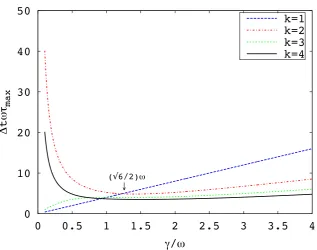
6. Figure2indicates that, for fixed∆tandω, the maximizingτis eitherτmax(1) orτmax(2), depending on the 200

value ofγ. The optimal damping coefficient isγ= (

√

6/2)ω, for whichτmax(1) =τmax(2) =

√

6/(ω∆t).

201

7. The eigenfunction forτmax(1) is the linear polynomialωq. For such a preobservable, it may not seem 202

correct that the IAcT becomes arbitrary close to zero asγgoes to zero. This does not mean, however

203

that the variance goes to 0, because Eq. (1) is an asymptotic result, and the IAcT is a prefactor for

204

the leading order 1/Nterm in the expression for the variance. The next order 1/N2term would

205

dominate ifγwere very small. An order 1/N2error is characteristic of uniform sampling, which

206

would be the consequence of near-Hamiltonian dynamics. Also, linear polynomials are special

207

in that their expectation is independent of total energy, so it matters little that near-Hamiltonian

208

dynamics poorly samples different values of total energy.

209

8. The eigenfunction forτmax(2) is a specific linear combination ofω2q2−1 andp2−1. For quadratic

210

polynomials, the total energy does affect its expected value, which is why it is necessary thatγbe

211

large enough to sample different energies on a reasonable time scale.

212

5.1. The forward transfer operator

213

The forward transfer operator is

Fu=ρ−1e∆tLK(ρu) where

ρ(q,p)∝exp(−1

2p 2₋1

2ω 2_q2_). andLKis the Fokker-Planck operator [12, Eq. (10.1)–(10.3), (10.9)]

LKf =−p ∂ ∂qf+ω

2_q ∂ ∂pf+γ

∂

Therefore,

F =e∆tL where

Lf = 1

ρLK(ρf) =−p ∂ ∂qf +ω

2_q ∂

∂pf−γp ∂ ∂pf +γ

∂2 ∂p2f. Using the relationLf = 1_ρLK(ρf), it is easy to show that the adjoint

L†f =p ∂ ∂qf−ω

2_q ∂

∂pf−γp ∂ ∂pf+γ

∂2 ∂p2f. 5.2. Gamma for maximum spectral gap

214

Ref. [12, Ch. 10, Eqs.(1, 2, 3b, 9, 22, 52, 60, 71, 72, 74, 77, 78, 82, 83)] gives the eigenvalues ofLKas

µk,l =−

1

2(k+l)γ− 1

2(k−l)δ, k,l=0, 1, . . . , with eigenfunctions

ψk,l =ρ(q,p)1/2(k!l!δk+l)−1/2(√γ+B −

√

γ−A)k(−

√

γ−B+

√

γ+A)lρ(q,p)1/2, where

γ± = 1

2(γ±δ) and δ= q

γ2−4ω2,

with the radical sign denoting the principal square root, and operatorsA,Bdefined by

Af =−ω−1 ∂ ∂qf+

1

2ωq f, Bf =− ∂ ∂pf +

1 2p f.

The operatorL has eigenfunctionsρ(q,p)−1ψk,l(q,p) and the same eigenvalues; F has these same

215

eigenfunctions and has eigenvalues exp(∆tµk,l).

216

Fork+l=1, one hasµ0,1=−γ−,µ1,0 =−γ+and

ϕ0,1 = (γ−/δ)1/2(−p+γ+q)ρ(q,p), ϕ1,0 = (γ+/δ)1/2(p−γ−q)ρ(q,p).

In the caseγ± = 1₂γ,F has a double eigenvalueλ2 = λ3 =e−ω∆tbut one eigenfunction ϕ2(q,p) = 217

p−ωqand one generalized eigenfunctionϕ3(q,p) = q, satisfying(F −λ2)ϕ3 = ϕ2. This results in 218

behavior involving a linear combination of e−ωt_andte−ωt_. 219

The eigenvalue nearest 1 depends on∆t. For small enough∆t, it is exp(−γ−∆t), and the spectral

220

gap isω∆t+O(∆t2)forγ ≤ 2ω andω∆t(2ω/γ)(1+ (1−(2ω/γ)2)1/2)−1+O(∆t2)otherwise. To

221

maximize the spectral gap, chooseγto be no greater than 2ω, corresponding to an underdamped system.

222

5.3. Gamma for maximum IAcT

223

To obtainτmax, one needs eigenelements forG, given by Eq. (2) withF =exp(∆tL). Note that the 224

subspace of polynomials of degree≤kis closed under application ofLandL†_{. Moreover, this holds} 225

separately for subspacePk of odd polynomials of degree≤ kfor kodd and for subspacePk of even

226

polynomials of degree≤kforkeven. And it applies also to operatorsE,F,F†_{, andG. Hence, the} Pkare

227

eigenspaces ofrG. These eigenspaces can be further decomposed as follows. LetP0k=Pkfork<2, and

228

letP0k=Pk∩P⊥k−2fork≥2. The claim is thatP0kis an eigenspace, of dimensionk+1. To confirm this, it

229

G†_=GandGv∈

Pk−2. Letube a basis forP0kchosen so there are even functions ofpfollowed by odd

231

functions ofp. In particular,

232

u = [ωq, p]T,

u = [ω2q2−1, ωqp, p2−1]T,

u = [ω3q3−3ωq,(ω2q2−1)p,ωq(p2−1), p3−3p]T,

u = [ω4q4−6ω2q2+3,(ω3q3−3ωq)p,(ω2q2−1)(p2−1),ωq(p3−3p),p4−6p+3]T, fork =1, 2, 3, 4, respectively. The polynomials inωqand inpare modified versionsHek of Hermite

polynomials. We haveLu= Aufor some matrix of constantsA, given by

A= 

     

0 −kω ω −γ . ..

. .. . .. −ω kω −kγ



     

. (16)

(Cf. Risken (1984), Eqs.(10.96),(10.97) forLK.) We haveEu=0andF0u=Fu=exp(∆tA)u. Therefore, from Eqs. (13) and (14), one has

Ck=hF0ku,uTi=exp(k∆tA)hu,uTi, and

K=coth(−1

2∆tA)hu,u

T_i=coth(−1

2∆tA)C0. For each value ofk,τmaxis the maximum eigenvalue of

1 2

C₀−1coth(−1

2∆tA)C0+coth(− 1 2∆tA)

T

. (17)

As explained in Sec.3.1, if the basis functions are re-ordered so that those that are even functions ofp

233

precede those that are odd functions ofp, the eigenvalue problem splits into 2 nearly equal parts.

234

Fork=1,A=XΛX−1whereΛ=diag(−γ−,−γ+)and

X= "

ω ω

γ− γ+

# .

The covariance matrixC0=hu,uTi=diag(1, 1), and matrix (17) is diag(τ+,τ−)where

τ± = 1

δ

±γ±coth(1

2∆tγ−)∓γ∓coth( 1 2∆tγ+)

.

Using the identity coth(x±y) = (sinh 2x∓sinh 2y)/(cosh 2x−cosh 2y), one gets that the eigenvalues of matrix (17) are

τ± = sinh

(1₂∆tγ)±γsinh(1₂∆tδ)/δ cosh(1₂∆tγ)−cosh(1₂∆tδ) .

The greater ofτ±isτ+, and it is a straightforward exercise to show thatτ+is an decreasing function ofωas along as

In practice, a numerical integrator is used, whose step size is chosen so that∆tL=θwhereθis some fractional value, e.g., 1₂, and Lis the magnitude of largest eigenvalue of the Jacobian matrix of the right-hand side of the system of (first-order) stochastic differential equations. In particular,

ω∆t=θ ifγ≤2ω; (19)

otherwise, it holds thatω∆t<γ∆t/2. Hence, inequality (18) is more than satisfied. It is more complicated to analyze the behavior of values ofτfork>1, so we exploit the smallness ofω∆tandγ∆tto do an asymptotic analysis. From expression (17), one sees that forP0k, itsτmaxequalsτ

(k)

max+O(∆t)whereτmax(k) is the greatest eigenvalue of

− 1

∆t(C

−1 0 A

−1_C

0+A−T). (20)

Fork=1, one hasC0=diag(1, 1)andτmax(1) =2γ/(ω2∆t), corresponding to the eigenfunctionωq. For k=2, one has

A−1= 1 2γω2



 

−γ2−ω2 2γω −ω2

−γω 0 0

−ω2 0 −ω2



 ,

C0=diag(2, 1, 2), and the largest eigenvalue for expression (20) is

τmax(2) = _2∆1 t

γ ω2 +

2 γ+

s γ2 ω4 +

4 γ2

! ,

corresponding to an eigenfunction that is some linear combination ofω2q2−1 andp2−1. Againτmax(k) is a decreasing function ofωfor small enough∆t. For generalk, the size of the elements ofAin Eq. (16) increase withω, which suggests that for practical values of∆t, the largest eigenvalue for expression (20) decreases with ω. This can be confirmed numerically. To reduce the number of parameters, write A=−ωB(γ/ω), and rewrite expression (20) as

1 ω∆t(C

−1

0 B(γ/ω)

−1_C

0+B(γ/ω)−T). (21)

The valueτmax(k) is the largest eigenvalue of matrix (21), soγ∆tτmax(k) is a function only of the ratioω/γ.

235

Fig.1plots this quantity fork=1, 2, 3, 4, confirming thatτmax(k) is decreasing function ofωfor fixed values

236

ofγand∆t. Therefore, for a multidimensional quadratic potential,τmaxis very likely to be determined 237

by the lowest frequency mode. (This is readily established for the spectral gap for reasonable values of

238

∆t.)

239

Having established that the lowest frequency mode is most likely responsible forτmax, letωdenote

240

the lowest frequencyω1, and consider the optimal choice ofγ. From matrix (21), observe thatω∆tτmax(k) 241

is a function only ofγ/ω. Accordingly, we chooseγ/ωto minimize maxkω∆tτmax(k). However,∆tmay 242

depend onγ, but only ifγ>2ων, according to Eq. (19). Let us initially ignore this possibility and revisit 243

it after determining the optimalγ.

244

Assuming that the maximum ofω∆tτmax(k) is attained fork = 1 ork = 2, there are two possible 245

locations for the bestγ. One is the choiceγ=

√

2ω, for whichω∆tτmax(2) =1+

√

2 andω∆tτmax(1) =2

√

2.

246

The other is the choiceγ= (

√

6/2)ωwhereω∆tτmax(k) =

√

6 for bothk=1 andk=2. The latter is the

247

better choice. This and the assumption that the maximum occurs fork<3 is supported by Fig.2. Since

248

(√6/2)ω₁<2ων, we see from Eq. (19) that there is no concern about∆tlimiting the value ofγ. 249

Note that for the optimalγ, the dynamics is underdamped in every mode.

10

10

10

10

10

0

0.5

1

1.5

2

∆

t

γτ

ω/γ

k=1

k=2

k=3

k=4

Figure 1.γ∆tτmax(k) vs.ω/γfork=1, 2, 3, 4

0

10

20

30

40

50

0

0.5

1

1.5

2

2.5

3

3.5

4

∆

t

ωτ

max

γ

/

ω

k=1

k=2

k=3

k=4

↓

(√6/2)ω

6. Discussion and Conclusions 251

It is asserted in the literature [1,3] that for comparing MCMC propagators and for ensuring

252

reasonably reliable simulation results, it is of great value to estimate the maximum autocorrelation

253

time over all possible observables. Certainly, this would seem desirable for comparing propagators, since

254

it is best to assume as little as possible about the actual observables that are to be estimated from the

255

Markov chain. Also, the longest IAcT would be most reliably estimated, because its accurate estimation

256

would call for a greatest number of samples; moreover, the accuracy of estimates of other IAcTs might

257

be influenced by the longest IAcT. Unfortunately, estimating IAcTs and assessing such estimates is a

258

difficult task, which could benefit greatly from further research.

259

In this article, it is suggested that the maximum IAcT be estimated by considering an arbitrary linear

260

combination of basis functions chosen to capture the lowest frequency motions of the dynamics of the

261

MCMC chain. Also appealing is the approach based on a set of well chosen indicator functions [10].

262

Another quantity for measuring performance of an MCMC propagator is the spectral gap. It

263

is related to equilibration time, but as a predictor of IAcTs, it can be arbritarily too pessimistic or

264

optimistic. This may occur for irreversible propagators applied to energy landscapes where entropy

265

barriers dominate energy barriers.

266

Shorter integrated autocorrelation times are thus a primary consideration in the design of MCMC

267

propagators. To this end, it is advantageous not to insist on reversibility. In particular, the ballistic

268

component of propagators like hybrid Monte Carlo and Langevin dynamics may offer dramatic speedups

269

for overcoming entropy barrriers, though no advantage for energy barriers.

270

Irreversible propagators typically have a parameter that determines the extent of diffusive behavior.

271

For discrete Langevin dynamics applied to a multidimensional quadratic potential, the optimal value

272

corresponds to slightly underdamped dynamics for the lowest frequency mode, with other modes

273

experiencing even lighter dampling. Although this conclusion is not necessarily indicative of the optimal

274

damping for the usual situation, in which there a multiplicity of energy minima, it can be helpful to

275

begin with an understanding of simple situations.

276

Author Contributions:Y.F. performed the analysis for Sec.5.2and the computation for Sec.5.3. R.S. did the analysis

277

for Secs.3.1,4,5.1,5.3and wrote the paper.

278

Conflicts of Interest:The authors declare no conflict of interest.

279

280

1. Fang, Y.; Cao, Y.; Skeel, R. Quasi-Reliable Estimates of Effective Sample Size, 2017. arXiv:1705.03831v2

281

[stat.CO].

282

2. Schütte, C.; Huisinga, W. Biomolecular Conformations as Metastable Sets of Markov Chains. Proceedings of

283

the 38th Annual Allerton Conference on Communication, Control, and Computing, 2000, pp. 1106–1115.

284

3. Lyman, E.; Zuckerman, D.M. On the Structural Convergence of Biomolecular Simulations by Determination

285

of the Effective Sample Size. J. Phys. Chem. B2007,111, 12876–12882.

286

4. Rey-Bellet, L.; Spiliopoulos, K. Irreversible Langevin Samplers and Variance Reduction: a Large Deviations

287

Approach.Nonlinearity2015,28, 2081–2104.

288

5. Leimkuhler, B.; Matthews, C. Rational Construction of Stochastic Numerical Methods for Molecular Sampling.

289

Appl. Math. Res. Express2013, pp. 34–56.

290

6. Leimkuhler, B.; Matthews, C.; Stoltz, G. The Computation of Averages from Equilibrium and Nonequilibrium

291

Langevin Molecular Dynamics. IMA J. Numer. Anal.2016,36, 13–79.

292

7. Geyer, C.J. Practical Markov Chain Monte Carlo. Stat. Sci.1992,7, 473–511.

293

8. Priestly, M.B.Spectral Analysis and Time Series; Academic Press, 1981.

294

9. Goodman, J. Acor, Statistical Analysis of a Time Series, 2009. http://www.math.nyu.edu/faculty/goodman/ 295

software/acor/,https://github.com/dfm/acor.

296

10. Zhang, X.; Bhatt, D.; Zuckerman, D.M. Automated Sampling Assessment for Molecular Simulations Using

297

the Effective Sample Size. J. Chem. Theory Comput.2010,6, 3048–3057.

11. Diaconis, P.; Holmes, S.; Neal, R.M. Analysis of a Nonreversible Markov Chain Sampler. Ann. Appl. Probab. 299

2000,10, 726–752.

300

12. Risken, H.The Fokker-Planck Equation. Methods of Solution and Applications; Vol. 18,Springer Series in Synergetics,

301

Springer, 1984.