Feasibility of virtual environments to develop future driving cycles

2018-01-1816

Feasibility of Virtual Environments to Develop Future Driving Cycles

Peter Kay

University of the West of England

Abstract

The current procedure for testing emissions from new vehicles, the World Harmonised Light Vehicle Test Procedure (WLTP), was introduced in September 2017. The WLTP was developed by collecting over 765,000 kilometres worth of data in order to isolate driver behaviour from other real world variables. However, this is a very time consuming and costly process. This paper discusses the suitability of a cheaper and more time efficient alternative.

Driver behaviour has a significant impact on the emissions produced from the same vehicle. This study explores the feasibility of utilising virtual environments as an alternative to real world testing to isolate driver behaviour to develop future drive cycles. The use of virtual environments have some significant advantages over real world testing: they can be strictly controlled in terms of the weather, topography and vehicle characteristics, thereby aiding the isolation of driver behaviour from other variables.

A driving simulator facility based at the University of West of England was used to assess the suitability of determining driver behaviour using a virtual environment. A track was created based on a local route in the virtual environment. The virtual route was driven by volunteers and their driving behaviours were identified. The same route in the real world was driven by the same volunteers. The driving behaviour of the volunteers from both the virtual environment and the real world are compared to assess the realism of the virtual driving experience in terms of driver behaviour. Finally the data from the virtual environment were analysed to determine if driver behaviour can be isolated, along with the impact on vehicle emissions, with a view to using virtual environments to develop future drive test cycles for emissions testing.

Introduction

The New European Driving Cycle (NEDC) was replaced in 2017 by the World Harmonised Light Test Procedure (WLTP). The NEDC, as shown in Figure 1a, was widely criticised for not accurately reflecting real world driving [1, 2], in particular the main criticisms were:

 Low accelerations

 Constant cruise speeds

 Many idling events

The WLTP was developed to address these criticisms. To develop the WLTP data were collected from 13 countries across three continents totalling over 765,000 km worth of data [3]. Such a large amount of

data were collected in order to isolate the driver behaviour from all the other factors such as topography, local traffic conditions, weather conditions and local highway codes and etiquette. The WLTP is shown in Figure 1b.

0 200 400 600 800 1000 1200 1400

0 10 20 30 40 50 60 70 80 90 100 Time [s] V el o ci ty [ kp h ] (a)

0 200 400 600 800 1000 1200 1400 1600 1800 2000 0 20 40 60 80 100 120 140 Time [s] V el o ci ty [ kp h ] (b)

Figure 1. Variation of velocity with time for (a) New European Driving Cycle and (b) World Harmonised Test Procedure

Figure 2 shows the percentage change in vehicle horsepower [4], weight [4] and stopping distance from 70 mph [5] since 1975. Over that time the power to weight ratio has increased, on average, by 1.5% per annum. The stopping distance, over a 30 year period, has decreased at an average rate of 0.5% per annum. Between 1997 and 2017, the period where the NEDC was implemented, the power to weight ratio of the vehicles has increased by 20%. Therefore, an argument can be made that within a short period of time after implementation a drive cycle is no longer applicable to the vehicles being tested by the cycle, due to advances in vehicle and powertrain technology.

1970 1980 1990 2000 2010 2020 -25 -20 -15 -10 -5 0 5 Horsepower Weight Stopping Distance Year [-] P er ce nt ag e ch an ge s in ce 1 97 5 [% ]

Figure 2. Variation of the percentage change in vehicle horsepower [4], weight [4] and stopping distance since 1975 [5].

A drive cycle should be representative of the vehicles that are currently on the market. However, if the current method of developing drive cycles, and the gap between new cycles, is continued then this is not achievable. This is compounded by the increasing development of vehicle manufacturers and hence the rate at which new vehicles, and vehicle technology, are released onto the market. For example, Volvo have announced plans to reduce the development time of their vehicles from 42 to 20 months [6]. Therefore there is a question about the applicability of the WLTP with regards to current vehicles and, especially, future vehicles.

Increasing levels of simulation are being adopted throughout the engineering industry. In a driving simulator, unlike the real world, the environmental aspects, such as weather conditions, traffic and topography, can be strictly controlled, making it easier to decouple the driver behaviour from the other variables [7, 8]. In this context the use of a simulator would reduce the time and cost of developing future drive cycles.

This paper uses a small scale pilot study to assess the feasibility of using a virtual environment to reduce the lead time of future drive cycles. In particular this paper addresses the following:

 Is the driver behaviour in a simulator the same as in the real world?

 Can individual driver behaviour be isolated in the simulator?

Methodology

To enable the suitability of the simulator to be evaluated the selected route had to meet certain criteria:

 Have a range of ‘corners’ and ‘straights’ to help evaluate a range of driver behaviours.

 Not too long in length, so that the virtual track could be created with a reasonable amount of resources.

 Have minimal other road users, to ensure a ‘clean’ run and allow easier comparison to the virtual environment.

An industrial park opposite the University of the West of England was selected that met the above criteria. The selected route allowed for a long and short route to be developed. The short route was around 1.2 km and the long route was 1.6 km. Both featured a combination of long stretches of road and some low-velocity sections around car parks.

Virtual Environment

The virtual environment was first created in Race Track Builder (http://www.racetrackbuilder.com/). The track was created by tracing satellite images of the route within the software. The local landmarks and surroundings could not be recreated exactly. Instead generic pre-existing buildings in the software were used to create the impression of the business park.

The track was then exported from Race Track Builder into Cruden Panthera simulator software (http://www.cruden.com/) via 3DS Max. Figure 3 shows a screenshot of the virtual environment from inside the Cruden Software.

Figure 3: Screen shot of virtual environment in Cruden Panthera

The virtual environment was loaded into the existing simulation facility at the University of the West of England. The facility has a 180° wrap-around screen and three projectors to create a seamless image, although for this study only one projector was used. The vehicle was controlled using a Logitech G920 steering wheel, pedals and manual gear shifter. The steering wheel offered force feedback to improve the realism. The simulator didn’t use any motion or any other vestibular cues.

Vehicles

Two vehicles were used to get assess the suitability of the simulator across multiple vehicles. The two vehicles used were a Hyundai i20 and a Skoda Fabia. The data for each vehicle are presented in Table 1.

Table 1. Comparison of vehicles used in during the real world tests.

Vehicle Hyundai i20 _{Skoda Fabia}

Registration Year 2013 2009

Emissions Regulations Euro 5 Euro 5

Fuel [-] Petrol Diesel

Engine Displacement [cc] 1396 1422

Mass [kg] 1131 1155

Maximum Torque [Nm]

(at speed [rpm]) 137 (4200) 195 (2200)

Maximum power [kW]

(at speed [rpm]) 74 (5500) 59 (4000)

Transmission [-] Manual Manual

Number of forward gears [-] 6 5

The data above were inputted into the virtual environment to change the vehicle characteristics in the simulator.

Real World Tests

Three volunteer drivers were selected to drive the route in the real world. Only one driver drove different tracks in different vehicles.

Real world engine telemetry from the vehicles were collected via the OBD2 port on the vehicle. An OBD2 adapter synchronised with a smart phone logged the data from the vehicle at a rate of 1 Hz. In addition to the engine, a dash-cam was used for each trip. The recordings were then used to clarify any discrepancy between the virtual and real word data. For example, the dash cam would record a pedestrian stepping out in front of the vehicle, explaining a harsh braking event in the data.

Drivers

All the three drivers in this short study were employees of the university and had full clean UK driving licenses.

Results

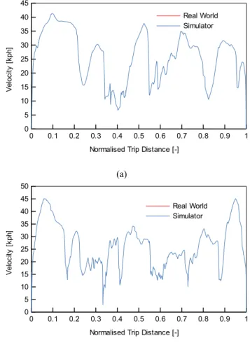
Figure 4 shows the variation of velocity against normalised trip distance for Driver 1. Figure 4a shows the data for the short route in the Hyundai and Figure 4b shows the data for the long route driven in the Skoda.

Due to a slight discrepancy in the length of the trip measured between the real world and the simulator. The trip distance was normalised against the cumulative trip distance. The error between the trip distances is small, 21 m in 1.2 km giving an error of 1.75%, and is due to slight errors in the generation of the virtual track.

0 0.1 0.2 0.3 0.4 0.5 0.6 0.7 0.8 0.9 1 0 5 10 15 20 25 30 35 40 45 Real World Simulator

Normalised Trip Distance [-]

V el oc ity [ kp h] (a)

0 0.1 0.2 0.3 0.4 0.5 0.6 0.7 0.8 0.9 1 0 5 10 15 20 25 30 35 40 45 50 Real World Simulator

Normalised Trip Distance [-]

V el oc ity [ kp h] (b)

Figure 4. Variation of vehicle velocity against normalised trip distance for Driver 1 driving (a) short route in the Hyundai and (b) long route in the Skoda.

Figure 4 shows that generally the driver behaviour from both the real world and the simulator, in terms of the overall velocity with distance, are in good agreement. Both the magnitude and the transient profile of velocity with distance correlate well.

The major difference between the real world and simulator is observed at around 10% through the long route (Figure 4a) and 15% through the short route (Figure 4b). At both these locations there is a significant deceleration and then acceleration in the real world that is not observed in the simulator data. The dash-cam footage shows that these relate to a speed bump that failed to be included in the virtual environment. It is proposed that the difference is due to the drivers slowing down, in the real world for the speed bump. It was not possible, within this study to repeat the simulation tests with the speed bump included.

Discussion

The data recorded from both the real world and the simulator for each driver were processed using the method outlined by de Haan and Keller [9]. The results for each driver are shown in the Appendix.

Real World v Simulator

Figure 5 shows the comparison of the average velocity and standard deviation of velocity for real world and simulation data for each driver using the method of de Haan and Keller [9].

Figure 5a shows that the change in average velocity for Drivers 1, 2 and 3 are 2.5%, -33% and 15% respectively. As discussed previously the average simulator velocity is expected to be higher due to the absence of the speed bump in the virtual environment.

1 2 3

0 5 10 15 20 25 30

Real World Simulator Driver [-] A ve ra ge V el oc ity [ kp h] (a)

1 2 3

0 2 4 6 8 10 12

Real World Simulator Driver [-] S ta nd ar d D ev ia tio n of V el co ity [ kp h] (b)

Figure 5. Comparison of (a) average velocity and (b) velocity standard deviation for real world and simulation data for each driver using the method of de Haan and Keller [9].

However, Driver 2 drove significantly slower, on average, in the simulator than in the real world. Driver 2 stated, after the test, that the simulator “made them feel uncomfortable”. ‘Simulator sickness’ is a known syndrome of using lab-based simulators to collect data. Simulator sickness can confound the data measured from the simulator [10]. It is suspected that Driver 2 suffered simulator sickness and therefore this could explain why there is a large discrepancy between the real world and simulator average velocities.

However, comparison of the average velocities between the real world and the simulator for Driver 1 and 3 are reasonably good.

Figure 5b shows the standard deviation for the velocity data. The maximum error between the simulator and the real world data is less than 10%. Interestingly, although there is a difference in the average vehicle velocity for Driver 2 due to simulator sickness, the standard deviation is comparable.

Figure 6 shows the comparison of average positive acceleration and average negative acceleration for real world and simulation data for each driver using the method of de Haan and Keller [9]

In general for both the real world and the simulator the average acceleration was approximately zero for all drivers, see Appendix. In other words the driver tended to accelerate as hard as they

decelerated.

1 2 3

0 0.1 0.2 0.3 0.4 0.5 0.6 0.7 0.8 0.9 1

Real World Simulator Driver [-] A ve ra ge P os iti ve A cc el er at io n [m /s 2] (a)

1 2 3

-1.2 -1 -0.8 -0.6 -0.4 -0.2 0

Real World Simulator Driver [-] A ve ra ge N eg at iv e A cc el er at io n [m /s 2] (b)

Figure 6. Comparison of (a) average positive acceleration and (b) average negative acceleration for real world and simulation data for each driver using the method of de Haan and Keller [9].

There are a number of factors that could contribute to this difference in average accelerations, such as the accuracy of the simulation environment, accuracy of the simulated vehicle and simulator feedback. Each of these factors will be discussed in turn.

As already discussed a speed bump was failed to be modelled in the simulator, this could have contributed to the difference in average acceleration. It was also noticed during the trials that the simulator trials that the turnings for the some of the corners were hard to spot, and hence resulting in a more cautious approach in the simulator.

Inaccuracies in the vehicle model in the simulator would also contribute towards a difference in acceleration. For example some of the parameters required by the simulator are hard obtain and so had to be estimated.

Perhaps the most important difference is that the simulator does not currently offer any vestibular or proprioceptive cues. Studies have shown that the lack of vestibular cues during lateral acceleration, especially braking, can lead to braking behaviours that differ from the real world [8]. This is certainly an area that is currently being considered for development. However, studies also report that in a static simulator the simulator behaviour can get close to the real world data by training the drivers, with just a few trials[11]. The drivers in the current study were not ‘trained’ in using the simulator, therefore it is anticipated that better acceleration comparisons could be obtained following a similar method of Jamson and Smith [11].

Individual Driver Behaviour

Figure 5a shows that there are significant differences between the individual driver behaviour of the individuals. The average simulator vehicle velocity of Driver 3 was 20% more than Driver 1. Figure 5b shows that there is also a marked difference between the standard deviation of the vehicle velocity. The standard deviation simulator velocity of Driver 3 was 30% more than Driver 2. This demonstrates that the individual driver behaviour can be isolated and used to develop a drive test cycle.

Conclusions

This paper presents a pilot study to assess the use of a simulator to develop future drive cycles. A track in the real world was identified and reproduced in the simulator. Three drivers drove the ‘track’ in the real world and in the simulator and data from both the vehicle and the simulator were recorded and compared. The main conclusions are:

 The transient velocity of each driver in the simulator accurately matched the real world data. Any major discrepancies are the result of features not included in the simulator, such as speed bumps.

 Data processed using the method of de Haan and Keller [9] broadly showed good agreement between the real world and the simulator velocity data, giving confidence that the driver behaviour is the same in the simulator as in the real world.

 The processed data highlighted significant differences between each of the drivers, emphasising the fact that individual driver behaviour can be isolated and used to develop future drive test cycles.

 Simulator sickness affected one of the volunteers confounding the data.

 There were major discrepancies between the average positive and negative accelerations of each driver in the simulator when compared to the real world. There are many factors that affect this and future studies aim to mitigate this using established techniques [11].

 Overall, the results show promise that simulators could be used to develop future drive test cycles, thereby resulting in a more time and cost-efficient solution.

Limitations

It should be noted that principally this study is a pilot study to examine the feasibility of using driving simulators to study real world driver behaviour. This has been successful, there are a number of limitations that prevent wider conclusions being drawn.

 The sample size is small with only three participants

 The sample were told about the research in advance and hence may have influenced their behaviour

 ‘Simulator sickness’, which is affects most simulation studies also affected one of the participants.

References

1. Dings, J., “Mind the gap! Why official car fuel economy figures don’t match up to reality”. Transport and Environment, Brussels (2013)

2. Mock, P., German, J., Bandivadekar, A., Riemersma, I., Ligterink, N. and Lambrecht, U., “From laboratory to road: a comparison of official and ‘real-world’ fuel consumption and CO2 values for cars in Europe and the United States”. International Council on Clean Transportation (2013) 3. Tutuianu, M., Marotta, A., Steven, H., Ericsson, E., et al,

“Development of a World-wide Harmonized Light Duty Test Cycle (WLTC)”. 2013. UN/ECE/WP.29/GRPE/WLTP-IG. 4. EPA, “Light-Duty Automotive Technology, Carbon Dioxide

Emissions, and Fuel Economy Trends: 1975 Through 2017”. 2018. EPA-420-R-18-001

5. Car and Driver. “Short Stoppers”. 2008.

https://www.caranddriver.com/features/rocket-sleds-the-best- performers-from-50-years-of-car-and-driver-testing-short-stoppers-page-4

6. SAE, “Volvo’s Rapid Strategy aims at 20-month vehicle development”, 2014. SAE Article: http://articles.sae.org/13621/. 7. Norfleet, D., Wagner, J., Alexander, K. and Pidgeon, P.,

“Automotive Driving Simulators: Research, Education and Entertainment”. SAE International. 2009-01-0533.

8. Pinto, M., Cavallo, V. and Ohlmann, T., “The Development of Driving Simulators: Toward a Multisensory Solution”, Le Travail Humain, 71 62-95. 2008.

9. De Hann, P. and Keller, M., “Modelling fuel consumption and pollutant emissions based on real-world driving patterns: the HBEFA approach”. Int. J. Environment and Pollution. 22(3) 240-258. 2004

10. Brooks, J., Goodenough, R., Crisler, M., Klein, N., et al, “Simulator sickness during driving simulation studies”. Accident Analysis and Prevention. 42 788-796. 2010.

Contact Information

For more information please contact:

Dr Peter Kay.

+44 (0)117 32 86068 [email protected]

Acknowledgments

I would like to acknowledge Jon Ormaechea Merida for his contribution in modelling some of the virtual environment.

I would also like to thank the volunteers who took part in this study.

Abbreviations

NEDC New European Driving

Cycle

WLTP World Harmonised Light

Appendix

Table 2. Summary of real world and simulator data for Driver 1 calculated using the method outlined by de Haan and Keller [9].

Parameter Real World Simulator Percentage Change

Distance [m] 1668 1726 3.5

Total Time [s] 267 270 1.0

Stop Time [s] 1 0 -100.0

Driving Time [s] 266 270 1.3

Acceleration Time [s] 75 131 75.2

Deceleration Time [s] 75 116 54.9

Cruise Time [s] 116 22 -81.1

% Time Stopped [%] 0.4 0 -100.0

% Time Driving [%] 99.6 100 0.4

% Time Accelerating [%] 28 49 73.6

% Time Decelerating [%] 28 43 53.4

% Time Cruising [%] 43 8 -81.3

Average Velocity [kph] 22.5 23.0 2.5

Average Driving Velocity [kph] 22.6 23.0 2.1

Velocity Standard deviation [kph] 8.3 8.7 4.4

Average acceleration [m/s2_{] 0.004 -5.39E-05 -101.5}

Average positive acceleration [m/s2_{] 0.930 0.550 -40.9}

Table 3. Summary of real world and simulator data for Driver 2 calculated using the method outlined by de Haan and Keller [9].

Parameter Real World Simulator Percentage Change

Distance [m] 1709 1735 1.5

Total Time [s] 320 481 50.5

Stop Time [s] 1 0 -100.0

Driving Time [s] 319 481 50.9

Acceleration Time [s] 99 234 136.2

Deceleration Time [s] 80 191 139.3

Cruise Time [s] 140 56 -59.9

% Time Stopped [%] 0 0 -100.0

% Time Driving [%] 100 100 0.3

% Time Accelerating [%] 31 49 57.0

% Time Decelerating [%] 25 40 59.1

% Time Cruising [%] 44 12 -73.4

Average Velocity [kph] 19.2 13.0 -32.5

Average Driving Velocity [kph] 19.3 13.0 -32.7

Velocity Standard deviation [kph] 7.6 7.0 -8.7

Average acceleration [m/s2_{] 0.000 -9.21E-04}

-Average positive acceleration [m/s2_{] 0.659 0.578 -12.4}

Table 4. Summary of real world and simulator data for Driver 3 calculated using the method outlined by de Haan and Keller [9].

Parameter Real World Simulator Percentage Change

Distance [m] 1707 1731 1.4

Total Time [s] 250 220 -12.0

Stop Time [s] 1 0 -100.0

Driving Time [s] 249 220 -11.6

Acceleration Time [s] 80 109 35.8

Deceleration Time [s] 67 92 37.0

Cruise Time [s] 102 20 -80.7

% Time Stopped [%] 0.4 100

-% Time Driving [-%] 100 49 -50.7

% Time Accelerating [%] 32 42 30.3

% Time Decelerating [%] 27 9 -66.9

% Time Cruising [%] 41 45 9.8

Average Velocity [kph] 24.6 28.3 15.2

Average Driving Velocity [kph] 24.7 28.3 14.7

Velocity Standard deviation [kph] 10.1 9.1 -9.6

Average acceleration [m/s2_{] 0.000 -1.50E-05}

-Average positive acceleration [m/s2_{] 0.927 0.573 -38.2}